Data Normalization Explained: Types, Examples, & Methods

Data quality is the key to success for any organization. If you don't have good data, you're essentially flying blind. Before you know it, productivity takes a hit, systems fail, and costs start to soar. IBM uncovered that poor data quality carries an annual price tag of $3.1 trillion for the U.S. economy. To combat these issues and boost your data quality, one of the most effective strategies is data normalization.

Data normalization is a versatile process aimed at minimizing errors and inconsistencies in data that can significantly undermine the efficiency and accuracy of data systems. It reduces redundancy and standardizes data to promote integrity and consistency across various fields, from database management to data analysis and machine learning.

In this guide, we'll break down the complex concept of data normalization and explore its types and applications to help you handle your data more effectively. But first, let's begin by discussing data anomalies.

What Are Data Anomalies?

Data anomalies refer to inconsistencies or errors that occur when you deal with stored data. These anomalies can compromise the integrity of the data and cause inaccuracies that do not reflect the real-world scenario the data is meant to represent.

In databases, anomalies are typically because of redundancy or poor table construction. In data analysis and machine learning, anomalies can arise from missing values, incorrect data types, or unrealistic values.

Regardless of the context, anomalies can significantly impact the consistency and integrity of data. They can cause inaccurate analyses, misleading results, and poor decision-making. Therefore, identifying and addressing data anomalies is a crucial step in any data-driven process.

Exploring Data Anomalies: A Focus on Databases, Data Analysis & Machine Learning

Data anomalies can originate from a range of sources and their impact can vary, often causing substantial complications if not addressed properly. Let’s talk about 2 broad categories where these anomalies are most prevalent and can cause major issues.

Anomalies In Databases

Image Source

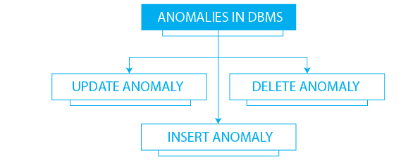
When it comes to databases, 3 primary types of data anomalies result from update, insertion, and deletion operations.

• Insertion anomalies: These occur when the addition of new data to the database is hindered because of the absence of other necessary data. This situation often arises in systems where specific dependencies between data elements exist.
  
• Update anomalies: This type of anomalies happen when modifications to the data end up causing inconsistencies. This usually occurs when the same piece of data is stored in multiple locations and changes aren't reflected uniformly across all instances.
  
• Deletion anomalies: You encounter these anomalies when you unintentionally lose other valuable information while removing certain data. This typically happens when multiple pieces of information are stored together and the deletion of one affects the others.

While the above anomalies are mainly related to the operations in databases and their design flaws, understand that anomalies are not limited to these aspects alone. They can very well be present in the data itself and can be a source of misleading analysis and interpretations. Let’s discuss these next.

Anomalies In Data Analysis & Machine Learning

In data analysis and machine learning, data anomalies can manifest as discrepancies in the values, types, or completeness of data which can significantly impact the outcome of analyses or predictive models. Let's examine some of the key anomalies that occur in this context: 

• Missing values: These happen when data is not available for certain observations or variables.
  
• Incorrect data types: These anomalies occur when the data type of a variable does not match the expected data type. For example, a numeric variable might be recorded as a string.
  
• Unrealistic values: This type of anomaly arises when variables contain values that are not physically possible or realistic. For example, a variable representing human age might contain a value of 200.

Now, let's look at the basics of data normalization and its significance in handling data anomalies. This vital aspect of data management and analysis ensures a more efficient process by standardizing data, eliminating redundancies, and addressing undesirable input errors. By mitigating the impact of anomalies, data normalization plays an important role in achieving reliable results.

Data Normalization: Understanding The Basics

Data normalization is an important aspect of data management and analysis that plays a crucial role in both data storage and data analysis. It is a systematic approach to decompose data tables to eliminate redundant data and undesirable characteristics.

The primary goal of data normalization is to add, delete, and modify data without causing data inconsistencies. It ensures that each data item is stored in only one place which reduces the overall disk space requirement and improves the consistency and reliability of the system.

In databases, it organizes fields and tables and in data analysis and machine learning, normalization is used to preprocess data before being used in any analysis.

Who Needs Data Normalization?

Data normalization has applications in a wide array of fields and professions. Its ability to streamline data storage, reduce data input error, and ensure consistency makes it an invaluable asset for anyone dealing with large datasets. Let’s discuss some of its use cases.

Data Normalization In Machine Learning

Data normalization is a standard preprocessing step in machine learning. ML engineers use it to standardize and scale their data which is very important to ensure that every feature has an equal impact on the prediction.

Data Normalization In Research

Researchers, particularly those in the field of science and engineering, often use data normalization in their work. Whether they're dealing with experimental data or large datasets, normalization helps to simplify their data, making it easier to analyze and interpret. They use it to eliminate potential distortions caused by differing scales or units and ensure that their findings are accurate and reliable.

Data Normalization In Business

In the business world, data normalization is often used in business intelligence and decision-making. Business analysts use normalization to prepare data for analysis, helping them to identify trends, make comparisons, and draw meaningful conclusions. 

This helps in more informed business decisions and strategies to drive growth and success. Normalization also improves data consistency which results in better collaboration between different teams within the company.

4 Types Of Data Normalization In Databases

Image Source

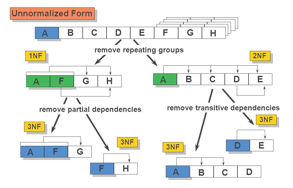
Data normalization in databases is a multi-stage process that involves the application of a series of rules known as 'normal forms'. Each normal form represents a level of normalization and comes with its own set of conditions that a database should meet. 

These normal forms give a set of rules that a database should adhere to for achieving a certain level of normalization. The process starts with the first normal form (1NF) and can go up to the fifth normal form (5NF), each level addressing a specific type of data redundancy or anomaly. Let’s take a look at each one of them.

1. First Normal Form (1NF)

The first normal form (1NF) is the initial stage of data normalization. A database is in 1NF if it contains atomic values. This means that each cell in the database holds a single value and each record is unique. This stage eliminates duplicate data and ensures that each entry in the database has a unique identifier, enhancing data consistency.

2. Second Normal Form (2NF)

A database reaches the second normal form (2NF) if it is already in 1NF and all non-key attributes are fully functionally dependent on the primary key. In other words, there should be no partial dependencies in the database. This stage further reduces redundancy and ensures that each piece of data in the database is associated with the primary key which uniquely identifies each record.

3. Third Normal Form (3NF)

The third normal form (3NF) is achieved if a database is in 2NF and there are no transitive dependencies. This means that no non-primary key attribute should depend on another non-primary key attribute. This stage ensures that each non-key attribute of a table is directly dependent on the primary key and not on other non-key attributes.

4. Beyond 3NF

While most databases are considered normalized after reaching 3NF, there are further stages of normalization, including the fourth normal form (4NF) and fifth normal form (5NF). These stages deal with more complex types of data dependencies and are used when dealing with more complex datasets. In most cases, however, ensuring data integrity and efficiency at the 3NF level is already sufficient.

3 Examples Of Data Normalization In Databases

To better understand these concepts, let's look into some practical examples of data normalization in databases.

A. First Normal Form (1NF) Example

Consider an employee table where employees are associated with multiple departments. The table is not in 1NF because it contains non-atomic values, i.e., cells with more than one value.

Employee Table

To achieve 1NF, we must split the data in the 'Department' column into 2 records, one for each department, so that each record in the table contains a single value.

Employee Table in 1NF

B. Second Normal Form (2NF) Example

Consider a Products table where the 'product' and 'brand' attributes are not fully dependent on the composite primary key 'productID' and 'brandID'.

Products Table

To bring the table to 2NF, we split the table into 3, where each non-key attribute is fully functionally dependent on the primary key.

Products Category Table

Brand Table

Products Brand Table

In the 'Product-Brand Link' table, each row represents a product-brand pair from the original table. This table effectively links the 'Products Category' table and the 'Brand' table, ensuring that the relationship between products and brands is maintained. Here’s the schema:

C. Third Normal Form (3NF) Example

Consider an Employee table where 'Salary' is dependent on 'Salary Slip No', which is not a primary key. This is a transitive dependency that is not allowed in 3NF.

Employee Table

To bring the table to 3NF, we split the table into 2 wherein each separate table, no non-primary key attribute depends on another non-primary key attribute.

Employee Table in 3NF

Salary Table

Data Normalization In Data Analysis & Machine Learning

Image Source

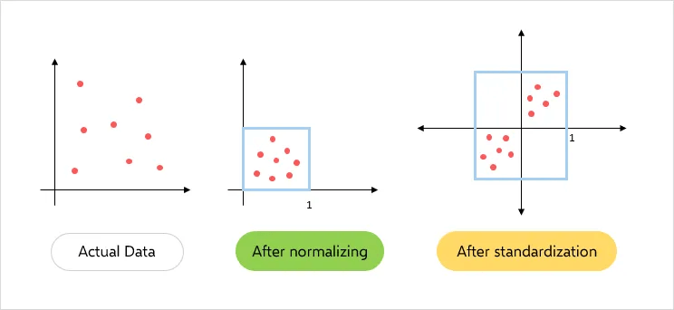
In data analysis and machine learning workflows, data normalization is a pre-processing step. It adjusts the scale of data and ensures that all variables in a dataset are on a similar scale. This uniformity is important as it prevents any single variable from overshadowing others.

For machine learning algorithms that rely on distance or gradient-based methods, normalized data is especially key. It helps these algorithms to function optimally and leads to the creation of models that are accurate, reliable, and unbiased. This ultimately enhances the quality of insights derived from the data.

3 Normalization Techniques & Formulas

Data analysis and machine learning use several techniques for normalizing data. Let’s discuss the 3 most commonly used methods.

Min-Max Normalization

This technique performs a linear transformation on the original data. Each value is replaced according to a formula that considers the minimum and maximum values of the data. The goal is to scale the data to a specific range, such as [0.0, 1.0]. The formula for min-max normalization is:

Z-Score Normalization

Also known as Zero mean normalization or standardization, this technique normalizes values based on the mean and standard deviation of the data. Each value is replaced by a score that indicates how many standard deviations it is from the mean. You can apply Z-score normalization using the following formula:

Decimal Scaling Normalization

This technique normalizes by moving the decimal point of values of the data. Each value of the data is divided by the maximum absolute value of the data, resulting in values typically in the range of -1 to 1. The formula for this simple normalization technique is:

3 Examples Of Data Normalization In Data Analysis & Machine Learning

Let’s apply the normalization techniques discussed above to real-world data. This can help us uncover the tangible effects they have on data transformation. We will use the Iris dataset which is a popular dataset in the field of machine learning. This dataset consists of 150 samples from 3 species of Iris flowers.

Here’s how you can import the data in Python:

python
from sklearn.datasets import load_iris
import pandas as pd

# Load the Iris dataset
data = load_iris()
x = data['data']
feature_names = data['feature_names']

# Create a DataFrame from the data for better visual representation
df = pd.DataFrame(x, columns=feature_names)

Here’s a sample of the dataset:

Min-Max Normalization Example

Min-Max normalization is a simple yet effective method to rescale features to a specific range, typically 0 to 1. Here is how you can perform Min-Max normalization using Python and Scikit-learn:

python
from sklearn.preprocessing import MinMaxScaler

# Create the scaler
scaler = MinMaxScaler()

# Fit and transform the data
df_min_max_scaled = pd.DataFrame(scaler.fit_transform(df), columns=df.columns)

When we apply Min-Max normalization to the Iris dataset, we get:

Z-score Normalization Example

Z-score normalization, or standardization, centers the data with a mean of 0 and a standard deviation of 1. Here's an example of how to perform Z-score normalization:

python
from sklearn.preprocessing importStandardScaler

# Create the scaler
scaler = StandardScaler()

# Fit and transform the data
df_standard_scaled = pd.DataFrame(scaler.fit_transform(df), columns=df.columns)

Z-score normalization of the Iris dataset gives:

Decimal Scaling Normalization Example

Decimal scaling normalization is particularly useful when the maximum absolute value of a feature is known. Here's a simple Python example of decimal scaling normalization:

python
import numpy as np

# Perform decimal scaling
max_abs_val = np.max(np.abs(df.values), axis=0)
df_decimal_scaled = df / 10 ** np.ceil(np.log10(max_abs_val))

The decimal scaling normalization code above first checks the order of the largest value in the dataset and then divides the entire dataset by it. Here’s the result:

The scales of the features in each of the 3 normalized datasets are much closer to each other than in the original dataset. This helps to ensure that all features contribute equally to the final result.

How Estuary Can Help With Data Normalization

Estuary Flow is a real-time data pipeline platform designed to facilitate the seamless ingestion, integration, and transformation of data in real time. It provides a robust infrastructure that lets users build and manage data pipelines with ease, ensuring that data is always up-to-date and readily available for analysis.

Flow is built on a foundation of open-source technologies and offers a unique approach to data management that combines the best aspects of traditional databases and modern streaming systems. Flow's architecture is designed to handle both batch and real-time data, making it a versatile tool for a wide range of applications.

One of the key ingredients of Flow is its use of collections, which are essentially real-time data lakes of JSON documents stored in cloud storage. These collections can either be captured from an external system or derived as a transformation of one or more other collections. This provides a flexible and efficient way to manage and normalize data.

Here are some of the key features of Flow that can support data normalization:

• Default annotations: It uses default annotations to prevent null values from being materialized to your endpoint system, ensuring data consistency.
  
• Real-time transformations: Flow supports SQL and Typescript for data manipulation, including functions like AVG(), MIN(), MAX(), and STDDEV() that can be used for data normalization.
  
• Projections: It uses projections to translate between the documents of a collection and a table representation. This feature is particularly useful when dealing with systems that model flat tables of rows and columns.
  
• Logical partitions: It allows you to logically partition a collection, isolating the storage of documents by their differing values for partitioned fields. This can help improve the efficiency of data storage and retrieval.
  
• Real-time data processing: It processes data in real-time which ensures that your normalized data is always up-to-date. This is particularly useful for applications that require immediate insights from the data.
  
• Reductions: Flow can merge multiple documents with a common key into a single document using customizable reduction strategies.
  
• Schema management: It uses JSON Schema to define your data’s structure, representation, and constraints. This allows for robust data validation and ensures that your data is clean and valid before it's stored or processed.
  
• Flexible data ingestion: Flow allows for the ingestion of data from a wide array of sources, including databases, cloud storage, and message queues. This flexibility makes it easier to bring in data from various sources for normalization.

Conclusion

Data normalization is a critical process in data management and analysis that ensures the integrity and reliability of data. However, the process can be complex and time-consuming, especially when dealing with large datasets and various types of anomalies.

This is where Estuary Flow comes in. It facilitates seamless real-time data operations and ensures that your data is always up-to-date and ready for analysis. With features like schema management and support for data manipulation functions, Flow can streamline the data normalization process.

So, if you're looking for a platform to simplify your data normalization process, you can explore Estuary Flow for free by signing up here or reaching out to our team to discuss your specific needs.