In the 2020’s, MapReduce isn’t a processing model that will turn many heads. It’s been around for well over a decade, and is easy to write off as an idea that might’ve been groundbreaking in its time, but is dated today.
MapReduce was a big deal for a reason, though, and it has a lot to offer, even now. When we incorporate new capabilities (like real-time processing) into this tried-and-true framework, we can overcome old pain points and reap the full benefits.
MapReduce then and now
MapReduce was introduced in a 2004 paper, which described the method used by Google to perform large-scale analytics using huge clusters of machines. By 2007, Apache Hadoop, the most well-known MapReduce engine, was at the beginning of its legendary hype cycle. To many, MapReduce is Hadoop. But Hadoop is just one implementation. Other systems like CouchBase and MongoDB also used map-reduce as a query engine.
Hadoop made a big splash, but these days it’s pretty niche in practice. That’s not because MapReduce itself is outdated, but rather because the problems that it solves are situations we now try to avoid. Hadoop is great when you want to do all your processing on one big cluster, and the data is already there. Of course, getting data into and out of that cluster can be a major issue, especially since these aren’t typically the system of record.
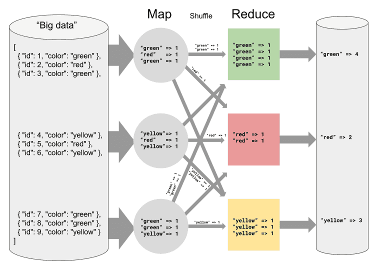
But the real problem is that traditional MapReduce is a “batch” processing framework, and that probably isn’t what you want in the first place. The basic premise is that you start by having “all” your data in the Hadoop cluster, then you run a job that executes a distributed computation over that data and spits out an answer.
But there’s no such thing as “all” your data. New data is generated constantly, and something’s always getting updated or corrected. “All your data” really just means “all the data that we know about so far.” So the best answers you can get from Hadoop are based on what was known at the time the job was run — and that time lag can be significant.
When data is added or updated, you need to first reconcile it with the data that’s already in your cluster, and then re-run the job to get the updated results. The more data there is, the longer this takes, so your jobs tend to get slower and slower as they churn through ever-growing sets of historical data.
This doesn’t mean we should abandon MapReduce — we simply need to move beyond the idea of it being just for batch processing.
MapReduce advantages for real-time data
To get the most out of your data the answers need to be timely, and data consumers are justifiably starting to expect that they can get information in real time.
Hadoop may not be the single solution to all your data problems (it never claimed to be), but the properties of MapReduce that made it desirable in the first place are still really useful in real-time data processing.
- MapReduce is a programming model that affords easy horizontal scaling. It’s easy to add nodes without requiring any changes to how the data is stored. This means that it’s able to cope with the huge growth in data volumes, which shows no sign of slowing down.
- MapReduce has a really simple and robust fault-tolerance model, which is critical when you start operating things at scale. It wouldn’t do any good to parallelize your transformation across 100 nodes if you couldn’t easily recover from the failure of one of them. After all, the more nodes you have, the more likely it is for any one of them to fail.
- Reduce functions are pure, which affords a ton of flexibility in when and where you run them. You could reduce eagerly or lazily, on the same node or a different one. As long as you apply the same inputs in the same relative order, you’ll get exactly the same results.
The flexibility of reduce functions is especially useful when reducing entity updates over time. Say you have a temperature sensor that produces readings, and you want to compute the minimum, maximum, and average temperatures. This is pretty straightforward with any MapReduce implementation.
Here’s a high-level overview of how it works.
Say you have input records that look like:
plaintext{"sensorId": "A", "timestamp": "2021-01-05T09:57:00Z", "tempC": 10.7}The map function might look like the following pseudocode:
plaintextfunction map(reading) {
    emit(reading.sensorId, {"timestamp": reading.timestamp, "min": reading.tempC, "max": reading.tempC, "current": tempC, "total": reading.tempC, "count": 1})
}
If you’re wondering why min, max, and total are all just set to the tempC of the input, it’s because those values will be updated as they are reduced with other values. The reduce function might look something like:
plaintextfunction reduce(left, right) {
    let result = {
        "min": math.min(left.min, right.min),
        "max": math.max(left.max, right.max),
        "total": left.total + right.total,
        "count": left.count + right.count
    }
    if (right.timestamp.isAfter(left.timestamp)) {
        result.current = right.current
        result.timestamp = right.timestamp
    } else {
        result.current = left.current
        result.timestamp = left.timestamp
    }
    return result
}
Now let’s say you have a series of sensor readings:
plaintext{"sensorId": "A", "timestamp": "2021-01-05T09:57:00Z", "tempC": 10.7}
{"sensorId": "A", "timestamp": "2021-01-05T09:58:00Z", "tempC": 10.8}
{"sensorId": "A", "timestamp": "2021-01-05T09:59:00Z", "tempC": 10.8}
{"sensorId": "A", "timestamp": "2021-01-05T10:00:00Z", "tempC": 11.0}
There’s multiple ways that you could reduce the mapped results. One way would be:
plaintextreduce(mapped[0], reduce(mapped[1], reduce(mapped[2], mapped[3]))). Another way would be:
plaintextreduce(reduce(mapped[0], mapped[1]), reduce(mapped[2], mapped[3]))Either way, you get the same results. Once you’ve passed all the records for a given sensor through this reduce function, the last output will contain your final answers.
Reduction is typically done incrementally, even in Hadoop. Say the computation is being done in parallel in multiple processes. Each process reduces all of its share of the values. The results from each separate process are subsequently reduced again with the results from the other processes to produce the final answer.
What’s interesting here is that reduction is fundamentally incremental. In batch processing systems like Hadoop, this property of reduction is used to incrementally aggregate the results of parallel computations from multiple processes. But when the input data is interpreted as updates to an entity over time, reduction gets even more useful.
In the example above, the entity is the sensor, and each is identified by a unique id. The readings can each be seen as updates over time. You might have each sensor perform some reductions itself in order to minimize the number of network calls (or to keep from losing data in the event that network connectivity is lost). Alternatively, data could be reduced at an edge node, and only aggregated results would ever need to be sent to your data warehouse. A more common and realistic scenario would be to simply delete older and low-value data and only retain the reduced values. The reduced values could then be used whenever new data arrives. So your job could conceptually involve something like: reduce(prevResults, reduce(newData...)).
Why MapReduce?
MapReduce allows the persistence and subsequent re-use of intermediate data. But why would you want that?
The basic answer is so that you can delete the original source data. That’s probably not important when you’re talking about things like purchase records, since you likely want to retain those for a long time anyway. But that kind of data, that’s worth storing in its original form for a long time, has become the exception rather than the rule.
Today’s organizations have access to way more data than they did five or ten years ago, but most of it isn’t high-value stuff like purchase records. For example, clickstream data coming from your website is really useful in the short term, but do you really want to store a record of every single click for years to come? Storage has gotten cheaper, but it’s definitely not free. This data is most useful within a fairly short time period, anyway, and quickly becomes less valuable. Maybe in the short term you want to retain the source data so you can drill down to specific examples of user interactions, but long-term you only want to store a per-user-session aggregate.
The other reason is that data pipelines are also getting more complex. This exacerbates the storage issues. When you have a pipeline that pulls in data from many different sources, it quickly becomes much less practical to store all of the original source data from each and every source. There are also laws like GDPR that limit the storage or accessibility of original source data. You need to instead store only aggregates of anonymized data, which introduces at least one additional layer of depth in your pipelines.
Imagine you have one job that processes the source data into some intermediate aggregate, and you can run that job whenever the source data is updated, say, daily, to process the new records and add to the intermediate results. Then you have other jobs that consume the intermediate results to produce increasingly complex aggregates. This actually works pretty well for MapReduce programs. Hadoop has long supported composing jobs in this way, such that the output from one is fed into the input of another.
But doing this with other paradigms typically comes with a lot more constraints. For example, a common approach is to aggregate intermediate results by some strict time window, like daily. So you take all the data from each day, output a daily result set, and then you roll up all the daily results into monthly, quarterly, or yearly reports. This has a number of big disadvantages. For one, it complicates the process of adjustments and corrections. Secondly, it limits the granularity with which you can update your final reports. If you aggregate intermediate results daily, you can’t see a partial day’s results.
Introducing continuous MapReduce
So what if we could adapt MapReduce to real-time data processing? (Spoiler: you can, it’s awesome, and it’s also the foundation of Estuary’s real-time data integration platform.)
The basic requirement is to change the concept of a “job,” and instead treat every MapReduce program as one that is continuously and incrementally updated.
Rather than producing output data and then exiting, like a Hadoop job, a continuous MapReduce program continues to update its results incrementally and in real time as new data is added. This means that it’s always fast and cheap to read the most up-to-date data. And updates and additions don’t require you to reprocess all the historical data! Furthermore, continuous MapReduce computations can be easily composed. You can easily feed the results of one computation into another computation as inputs, so even your most complex aggregates are updated incrementally in real time.
Continuous MapReduce works in much the same way as regular MapReduce, only without ever exiting. The main differences are the addition of a key extraction phase, and that the order of operations is a little different to facilitate the continuous, streaming execution.
In normal MapReduce, the map function emits arbitrary key-value pairs. The framework then has to shuffle these to the appropriate processes so that all the values for a given key will go to the same process. In continuous MapReduce, the key and value are extracted by separate functions, so it’s really more like key-MapReduce. Upon reading each record, the key is extracted by applying the key function. The record is shuffled to the appropriate process for that key. It is then transformed (mapped) by whichever member it got shuffled to, and the result of that transformation is reduced with the previous result(s) with the same key.
The same temperature sensor example using continuous MapReduce might look like this:
- Read a source record:
{"sensorId": "A", "timestamp": "2021-01-05T09:57:00Z", "tempC": 10.7} - Apply
key({"sensorId": "A", "timestamp": "2021-01-05T09:57:00Z", "tempC": 10.7})and get"A" - Shuffle the record to the appropriate process for
"A" - Apply
map({"sensorId": "A", "timestamp": "2021-01-05T09:57:00Z", "tempC": 10.7})and get{"sensorId": "A", "timestamp": reading.timestamp, "min": reading.tempC, "max": reading.tempC, "current": tempC, "total": reading.tempC, "count": 1} - Apply
reduce, passing in the previous result of the reduce function for key"A"and the result from the map function. - Repeat the previous steps whenever a new source record is available.
By this point, you’re probably wondering where the results of all these reductions are stored. After all, if we’re to keep running continuously and never exit, then we probably don’t want to hold all this data in memory forever. But the thing is that the set of keys and values is the output of the computation. It’s equivalent to the result set that’s output from a Hadoop job.
Estuary’s implementation of continuous MapReduce actually supports two different approaches for storing and retrieving these results. If the results are only intermediate and are just being fed into another continuous MapReduce computation, then we store them for you in partitioned and replicated stores backed by RocksDB. These are automatically co-located with the MapReduce process.
But you can also materialize the results to an external system that supports key-value semantics. In practice, this means that the results of reductions are stored in a database (like PostgreSQL) or a data warehouse (like Snowflake), which will be continuously updated as source data becomes available and flows through the system. The previous results will also be queried from this system so that updates can be reduced into them.
Consider the temperature sensor example again, this time with it being materialized into a Postgres table. After applying the map function, we look up the previous result for that key by querying it from the Postgres table. If present, the result is used as the left-hand-side input to the reduce function. Either way, the output is then persisted to the Postgres table, either by an update or an insert statement. This happens continuously, for each record read from the source (which may itself be just another continuous MapReduce). The Postgres table will always hold the most up-to-date results, and you never need to wait for a job to run.
Making old paradigms real-time
Our platform, Flow, uses continuous MapReduce as the foundation of its transformation runtime in exactly the way I just described. It’s a large part of the magic that powers the user-friendly web app most users see. In other words, continuous MapReduce lets you build real-time data pipelines without having to manage map, reduce, and key functions directly.
Across the industry, adapting tried-and-true frameworks for real-time processing is a growing, and promising, trend. We’ve all realized, in other words, that there’s no reason to reinvent the wheel. A prime example of this is the growing sector of streaming databases that offer creative takes on real-time SQL. Overall, it makes for a promising path forward into an era of real-time data processing.
We develop in the open, so if you’re interested and want to learn more about putting continuous MapReduce into practice, check out the source code on GitHub.
You can also sign up to try Flow for free and test the end result.

About the author
Philip Fried is a data infrastructure engineer focused on distributed systems, real-time pipelines, and scalable data movement.


