Snowflake Change Data Capture for AI

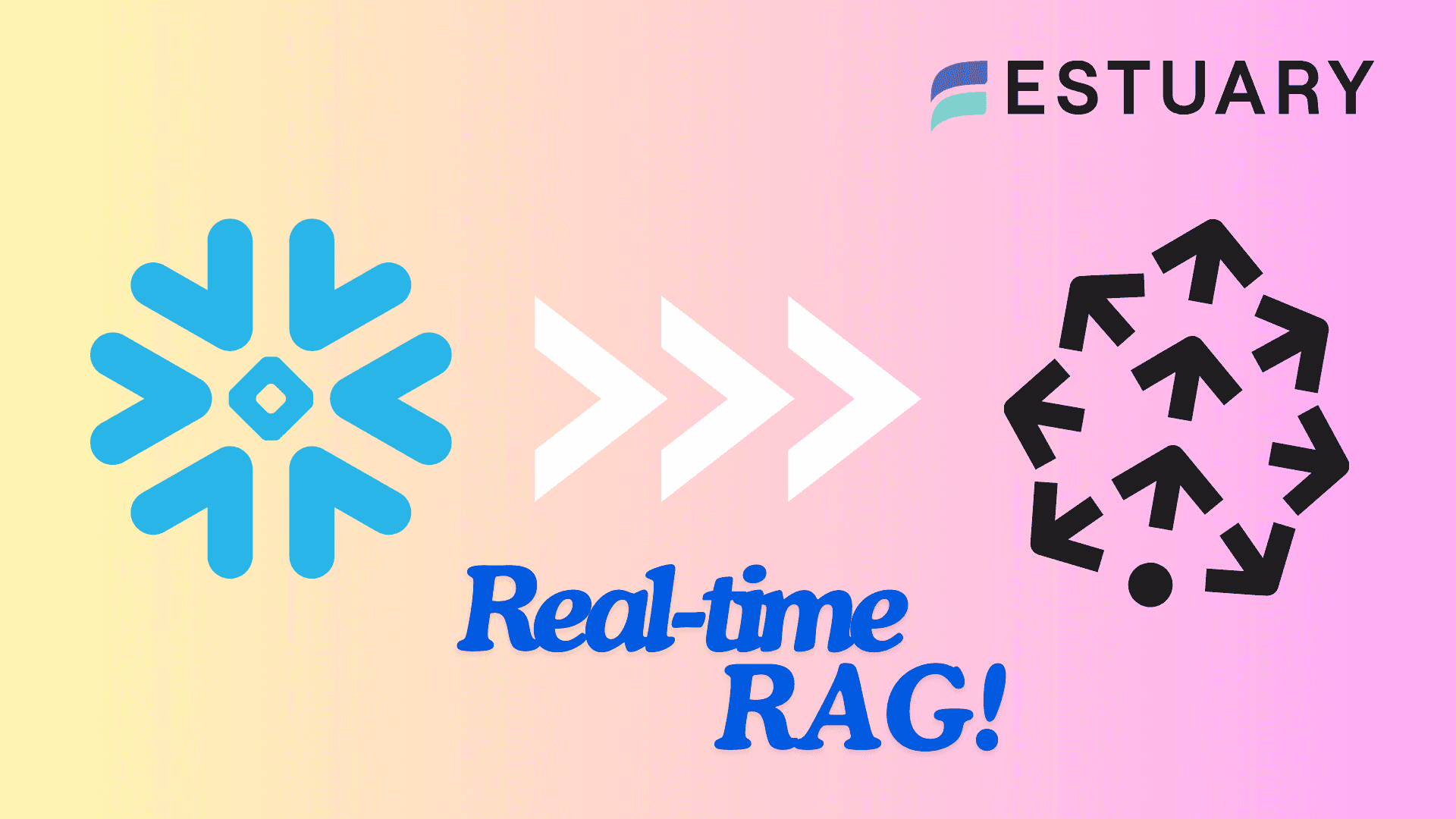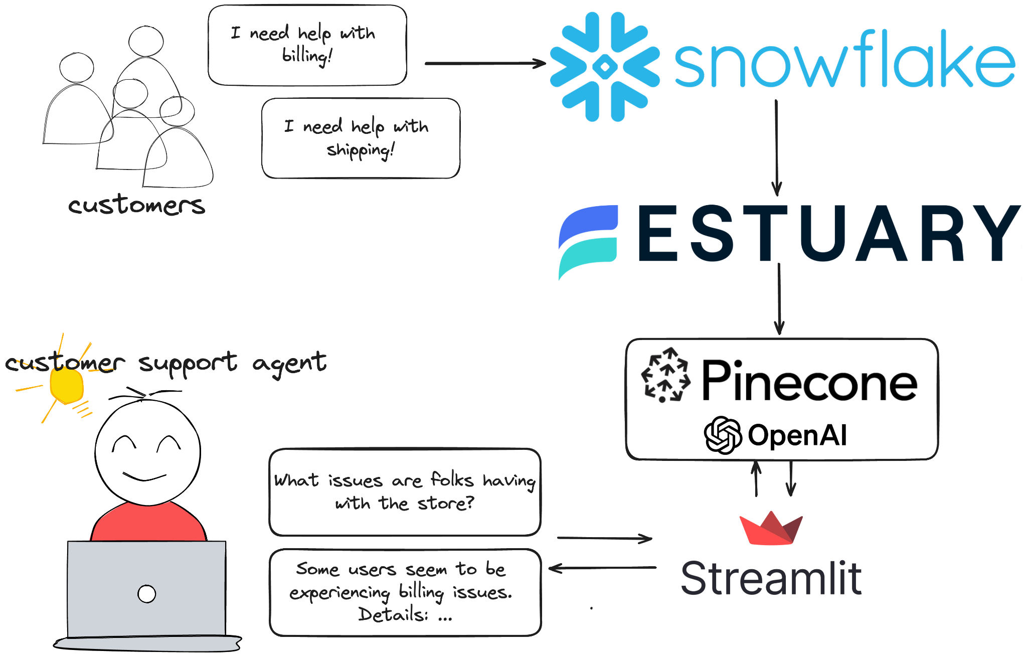
If you’re thinking about using Snowflake for AI, you don’t just need to get data into the warehouse, you also need to get data out of Snowflake, often in real-time. 

It’s actually pretty easy - you can use Snowflake as a change data capture (CDC) source!

In this article, after getting to know a few essential terms; you'll learn the following:

1. How to set capture change events from a Snowflake table
2. How to generate vector embeddings from the records and load them into Pinecone
3. And finally, how to implement a RAG-based ChatGPT-clone that can answer questions based on your data.

Let's get started!

What is CDC?

Change Data Capture (CDC) is a method used to track and capture changes made to data in a database. It allows for the real-time capture of insertions, updates, and deletions, creating a continuous stream of changes.

This data stream is crucial for keeping downstream systems synchronized with the source database. It enables real-time analytics, replication, and data integration. Essentially, CDC allows organizations to capture and react to data changes as they happen, ensuring data accuracy and timeliness across their systems.

If you’re interested in more, here’s an article with all the intricate details and best practices around CDC.

How does Snowflake do CDC?

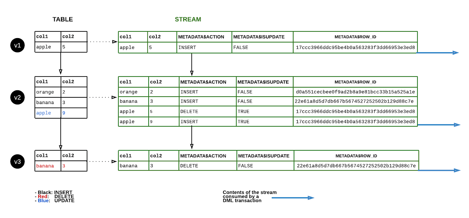
Snowflake Change Data Capture (CDC) uses streams to capture and track changes in real time. It is based on log-based data replication and captures changes in a source database, propagating them to a target database. A stream takes logical snapshots of a source object (such as external tables, tables, or views) and records DML changes to source objects in Snowflake, including updates, inserts, and deletes.

The Snowflake CDC process begins with creating a CDC-enabled table in the source database. Any changes made to this table are captured automatically and sent to the target database in near real-time.

After creating a stream for a table, new columns are added to the source table to store metadata that tracks data changes. Any data changes tracked by a stream must be consumed or moved to permanent storage within the set retention period, or a new stream will be created to track changes from that point forward.

Snowflake Streams, also known as table streams, are features of the Snowflake data warehouse platform that capture and track changes in data sources in real-time. They track all DML changes to the source table rows and store the metadata of each change.

A Snowflake stream takes an initial snapshot of every row of the source object, initializes an offset as the object’s current transactional version, and records DML-change information after this snapshot. Change records reflect the state of a row before and after the change, and include the source object’s column structure and additional metadata columns for describing each change event.

If you're keen to dive into the details of Snowflake CDC, you can check out this article for an in-depth explanation of the theory behind it. However, it's not a requirement for this tutorial, so feel free to keep reading to get started right away!

What is RAG?

Now that we know how we are going to get data out of Snowflake, let’s explore the wider architecture of our application.

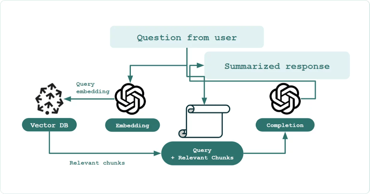
Retrieval-augmented generation (RAG) is a technique that combines search-based information retrieval with generative AI models. Generative models produce responses based only on existing training data, which may limit their accuracy and relevance over time.

In contrast, RAG dynamically retrieves relevant documents from external sources during the generation process. This approach ensures that responses are not only more accurate but also contextually relevant, especially when dealing with large datasets or when access to the latest information is crucial.

Understanding Vector Search

Vector search is a powerful way to find relevant data points by comparing their vector representations. In the context of RAG, vector search is essential for efficiently retrieving documents that are semantically similar to an input query. This process involves transforming data into high-dimensional vectors that capture the semantic meaning of the information.

Vector databases like Pinecone use these representations to perform fast and accurate similarity searches, enabling real-time, contextually relevant data retrieval that enhances the capabilities of generative models.

Imagine you are building a recommendation system for an online retail store. When a user views a product, the system converts the product's description into a vector representation. It then uses Pinecone to search for other product vectors that are semantically similar. This allows the system to recommend products that are contextually relevant to the user's interests.

For example, suppose a user is looking at a high-performance laptop. In that case, Pinecone can help identify and recommend other laptops with similar features, specifications, and reviews, thereby enhancing the shopping experience with personalized suggestions.

How Vector Search Works Using Pinecone:

1. Convert data into high-dimensional vectors.
   1. For example, product descriptions like "high-performance gaming laptop with 16GB RAM" and "ultra-thin laptop with 8GB RAM" are transformed into vectors using an embedding model. Each description becomes a point in a high-dimensional vector space.
2. Store these vectors in Pinecone.
   1. Each vector, along with its metadata (such as product ID, name, and description), is stored in Pinecone.
3. Convert the search query into a vector.
   1. When a user searches for "gaming laptop with good graphics", this query is also transformed into a vector using the same embedding model.
4. Perform a vector search to find similar vectors.
   1. Pinecone compares the query vector with the stored product vectors to find the most similar ones. The similarity is typically measured using distance metrics like cosine similarity or Euclidean distance.
5. Fetch the top results based on similarity.
   1. The most similar product vectors are retrieved, and their corresponding product details are returned to the user.

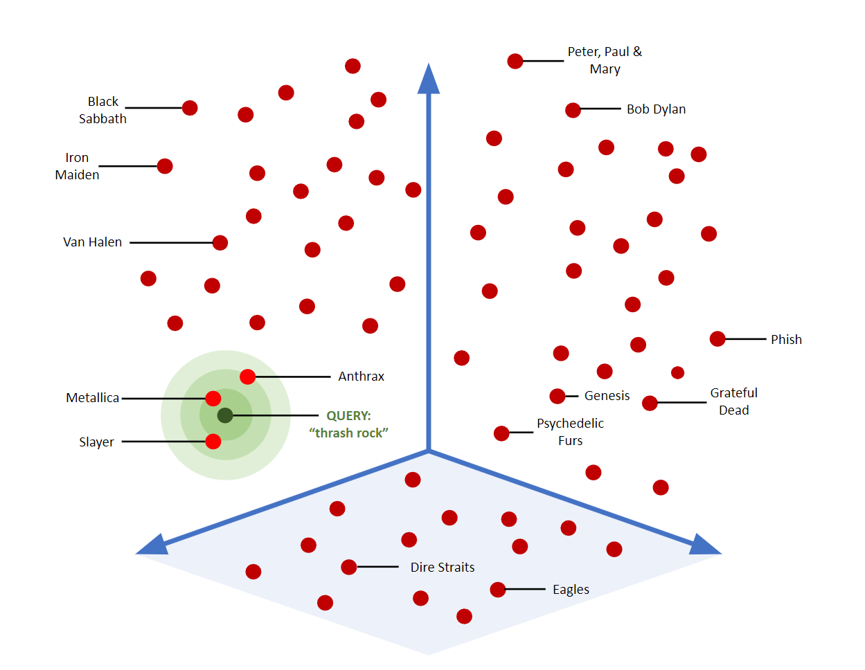
Consider the following visual representation of vector search in the context of metal bands:

• Vector Space: Imagine a multi-dimensional space where each point represents a metal band.
• Query Vector: A point in this space representing the search query, "thrash metal."
• Similarity Search: Green circles connecting the query point to the nearest points (bands) based on vector similarity.

In this illustration:

• The "Query" point represents the vector of the user's search query for "thrash rock."
• The "dot” marks represent vectors of different metal bands.
• The distance between the query point and band points indicates similarity. closer dots represent bands that are more similar to "thrash rock."

The Importance of Real-Time Contextual Data for RAG

Generative models have limitations because they are only as good as the data they were trained on. Large language models (LLMs) like GPT-4 are trained on huge datasets, but they may not include specific knowledge on topics such as finance, healthcare, technology, or current events.

For instance, a model trained a year ago may not be aware of recent advancements in AI, new scientific discoveries, or current geopolitical issues. This can result in outdated or inaccurate responses, reducing the usefulness of the model in providing timely and accurate information.

To address this, real-time data supplementation can transform generative models from static repositories of knowledge into dynamic sources of information. By continuously integrating new data, these models can adapt to changes and provide up-to-date responses.

This dynamic approach offers many benefits, for example:

• Models can generate responses reflecting the latest information, enhancing their accuracy and relevance. This is especially important in industries where outdated information can lead to costly errors.
• Organizations that use real-time data in their AI models can stay ahead of trends and make proactive, data-driven decisions, gaining a competitive edge. This capability can result in improved operational efficiency or better customer service.

So, how do we make a RAG system real-time? Continue reading to find out.

Introducing Estuary Flow

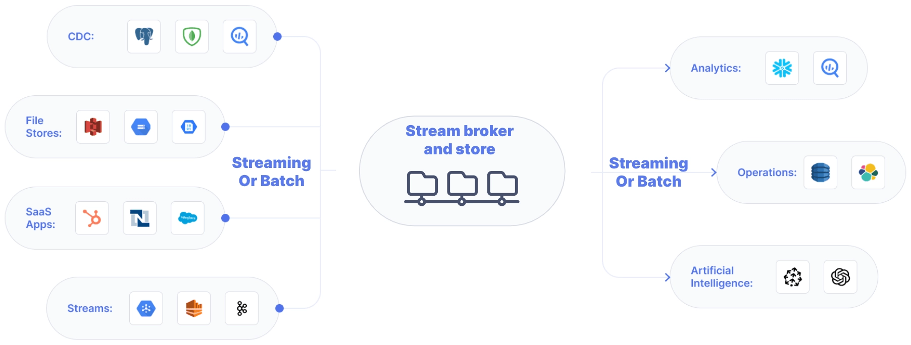
Estuary Flow is a real-time CDC platform built from the ground up for CDC and streaming. It excels at capturing data from various sources and delivering it to many destinations used for analytics, operations, and AI. With its event-driven architecture, Estuary Flow ensures data is processed and delivered exactly once, with low latency, making it an ideal solution to use with Materialize.

These capabilities are particularly beneficial for applications requiring continuous data updates, such as RAG implementations.

Some key features of Estuary Flow are:

• Fully Integrated Pipelines: Flow simplifies data integration by enabling you to create, test, and adapt pipelines that gather, modify, and consolidate data from multiple sources. 
• Change Data Capture (CDC): Always-on CDC that replicates in real-time with exactly-once semantics, backed by cloud storage.
• No-code Connectors: With pre-built connectors for popular data sources and sinks, such as databases and message queues, Flow reduces the need for custom connectors. This speeds up data pipeline deployment and ensures consistency across systems.
• Native support for vector databases like Pinecone, including the ability to vectorize data as part of the loading process.
• Support for real-time SQL, and TypeScript, including the ability to call APIs to use generative AI services like ChatGPT.

Tutorial Overview

The rest of the article will contain step-by-step instructions on how to build a real-time RAG application. You’ll learn how to:

1. Generate realistic-looking fake customer support ticket data into a Snowflake table.
2. Configure a Snowflake CDC capture in the Estuary Flow dashboard to ingest change events.
3. Set up a Pinecone Materialization to create vector embeddings from the incoming change events.
4. Spin up a simple Streamlit chat application for a clean conversational interface.

Prerequisites

• Estuary Flow account: if you haven’t registered yet, you can do so here, for free!
• Pinecone account: Pinecone is the target vector database in this project.
• OpenAI account: The project uses OpenAI’s API to calculate the embeddings and to wrap the chat responses using an LLM.
• Docker: for convenience, we provide a Dockerized development environment so you can get started in just seconds!

Step 1. Clone example repository and set up development environment

Head over to GitHub and clone the Estuary Flow examples repository. Change directories into the one called snowflake-cdc-pinecone-rag. This folder contains the data generator script and the Streamlit application for the chatbot.

Take a look at the docker-compose.yml file and make sure you update the environment variables before spinning up any containers. After you’re done, start the data generator script like this:

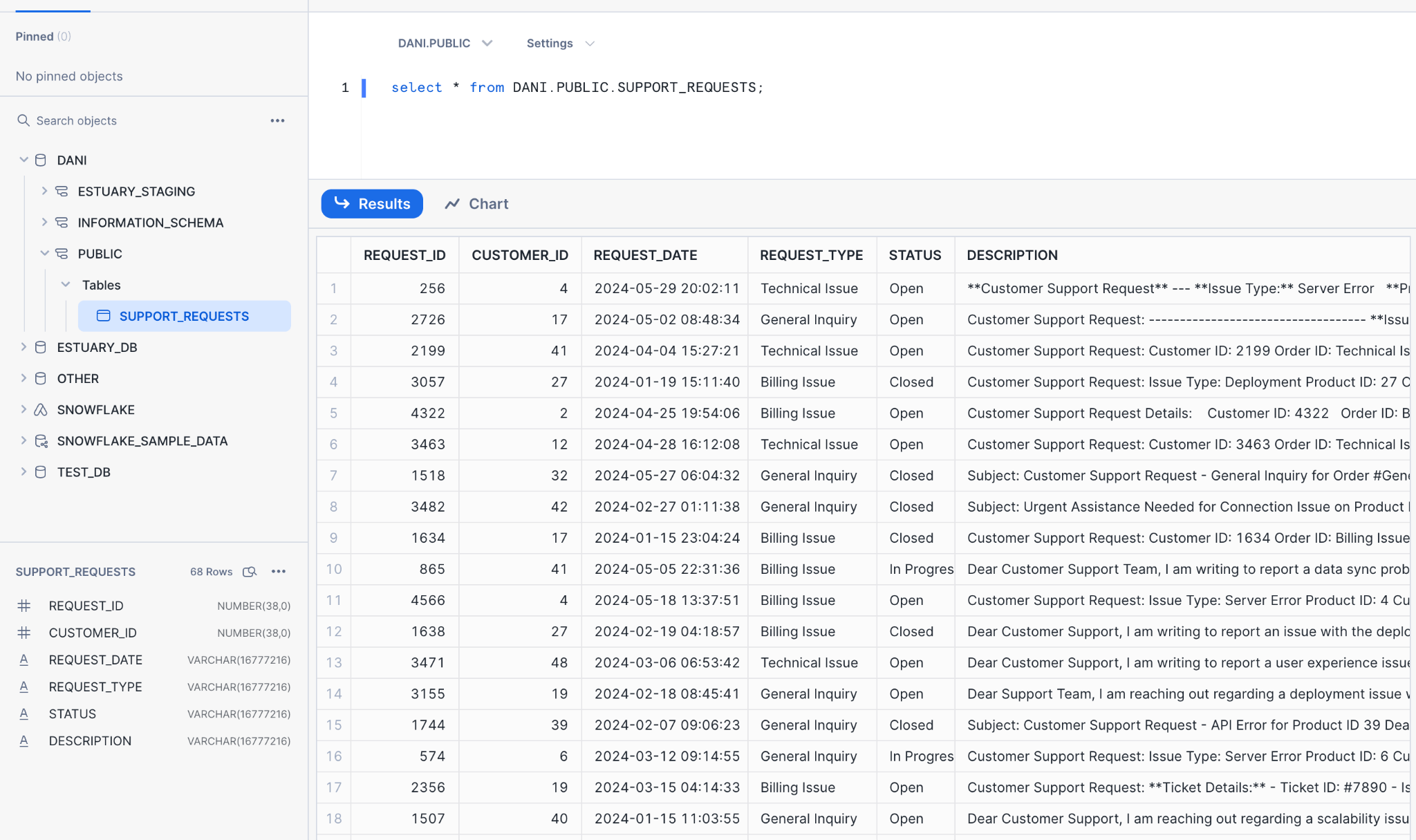
plaintext
docker compose up datagen

Head over to Snowsight to make sure data is being inserted into the table.

Perfect, this table contains fairly realistic-looking data thanks to the LLM-based data generator script, it will serve as a great data source for our RAG application.

Let’s move on to the next step, which is setting up Estuary Flow to capture changes to this table.

Step 2. Capturing Changes from Snowflake

To start streaming change events inside Snowflake using Estuary Flow's Snowflake CDC capture connector, you will need the following:

1. A target database containing the tables you want to capture data from.
2. A virtual warehouse that the connector can use to execute queries.
3. A schema to hold streams and staging tables managed by the connector. The default name for this schema is ESTUARY_STAGING unless overridden in the capture's advanced configuration.
4. A user with access grants for the necessary resources, as well as authorization to read from the desired source tables, and to create streams and transient tables in the staging schema based on the source tables.
5. The host URL for your Snowflake account. This is formatted using your Snowflake account identifier and might look something like sg31386.snowflakecomputing.com or df98701.us-central1.gcp.snowflakecomputing.com.

Here’s a script you can use to create all of these dependencies in one swoop!

plaintext
set database_name = 'DANI';              -- The database to capture from
set warehouse_name = 'ESTUARY_WH';       -- The warehouse to execute queries in
set estuary_user = 'ESTUARY_USER';       -- The name of the capture user
set estuary_password = 'secret';         -- The password of the capture user
set estuary_role = 'ESTUARY_ROLE';       -- A role for the capture user's permissions

-- Create a role and user for Estuary
create role if not exists identifier($estuary_role);
grant role identifier($estuary_role) to role SYSADMIN;
create user if not exists identifier($estuary_user)
  password = $estuary_password
  default_role = $estuary_role
  default_warehouse = $warehouse_name;
grant role identifier($estuary_role) to user identifier($estuary_user);

-- Create a warehouse for Estuary and grant access to it
create warehouse if not exists identifier($warehouse_name)
  warehouse_size = xsmall
  warehouse_type = standard
  auto_suspend = 60
  auto_resume = true
  initially_suspended = true;
grant USAGE
  on warehouse identifier($warehouse_name)
  to role identifier($estuary_role);

-- Grant Estuary access to read from all tables in the database and to create a staging schema
grant CREATE SCHEMA, MONITOR, USAGE
  on database identifier($database_name)
  to role identifier($estuary_role);
grant USAGE
  on future schemas in database identifier($database_name)
  to role identifier($estuary_role);
grant USAGE
  on all schemas in database identifier($database_name)
  to role identifier($estuary_role);
grant SELECT
  on future tables in database identifier($database_name)
  to role identifier($estuary_role);
grant SELECT
  on all tables in database identifier($database_name)
  to role identifier($estuary_role);

If you get stuck during the connector set up feel free to reach out to us on our Slack Community!

You will also need to enable change tracking on the table you wish to capture. You can do this by running the following:

plaintext
ALTER TABLE SUPPORT_REQUESTS SET CHANGE_TRACKING = TRUE;

Once these are in place, head over to your Estuary Flow dashboard.

1. Navigate to the "Sources" section.
2. Click on "Create New Capture".
3. Choose "Snowflake" as your capture connector.

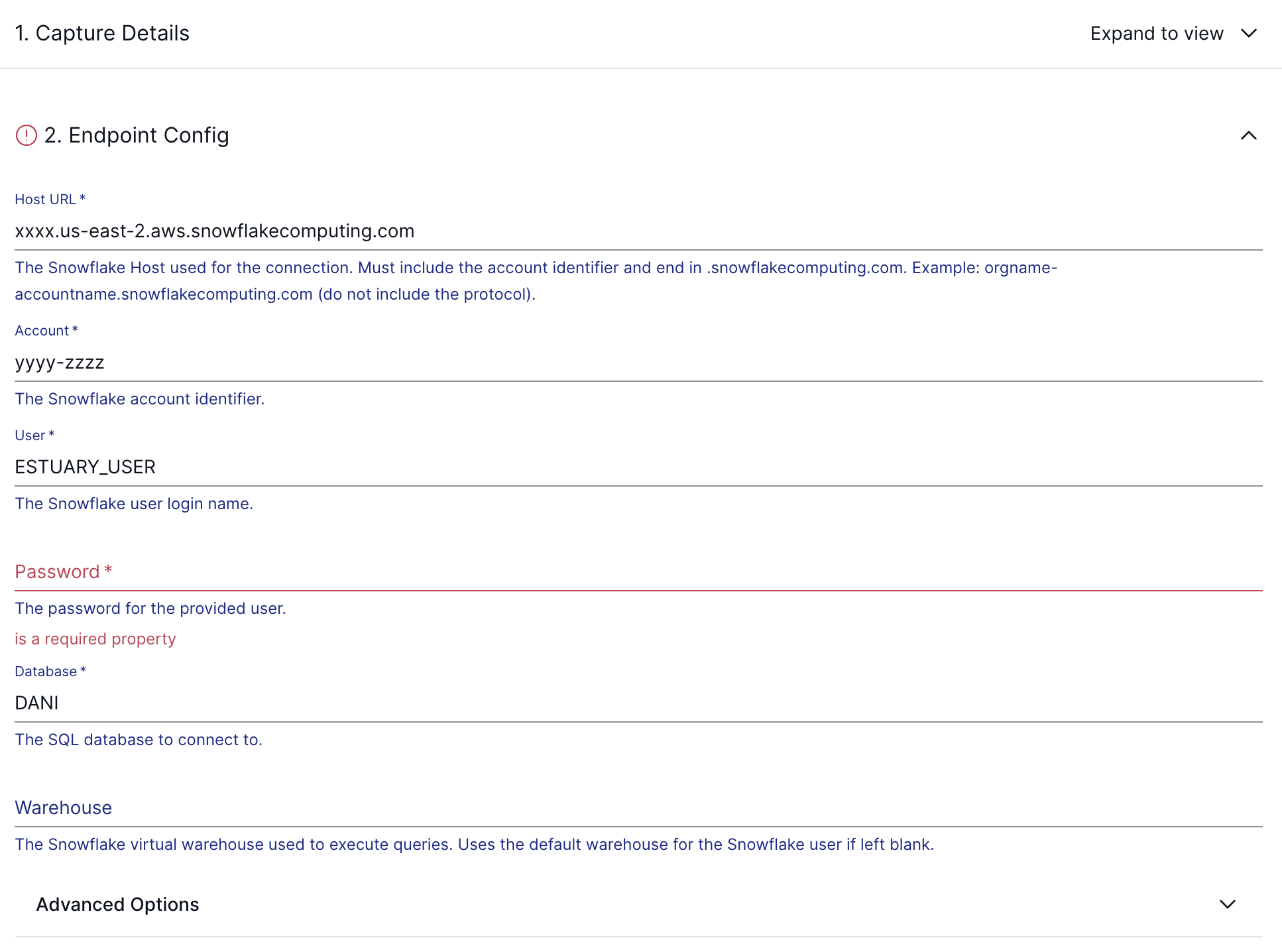
Configure the connection details based on your Snowflake environment.

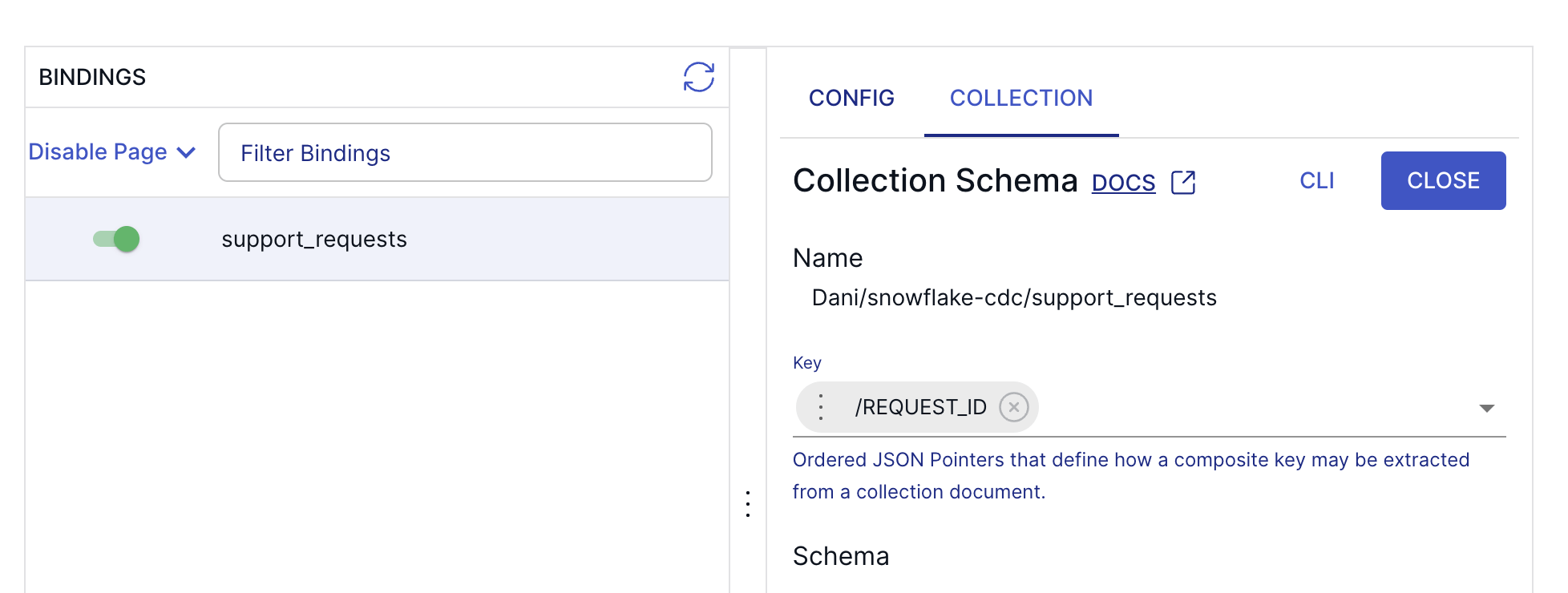
As a last step before publishing your capture connector, make sure you configure a Key for the Collection that the connector will use as its destination. In this case, it can be REQUEST_ID, the data generator script will make sure to not introduce duplicates.

And that’s it, press “Save and Publish”, and wait a few seconds until the automated backfill process gathers all existing records in the table.

An important note on polling intervals:

The Snowflake CDC connector captures changes at set intervals. The default interval is 5 minutes, balancing cost and capture latency. You can adjust the interval to reduce latency at the expense of higher costs. A longer interval reduces Snowflake costs but may result in lagging data capture. Regardless of the interval, the output collections will accurately represent the source tables up to a certain point in time.

The interval may be configured by editing the task spec interval property as described here.

Step 3. Vectorizing and Loading Data into Pinecone

Pinecone is a specialized vector database designed for high-performance vector search and similarity matching. By converting your tabular data from Snowflake into vectors and loading it into Pinecone, you can use its native search capabilities to quickly find relevant information.

To quickly set up Estuary Flow’s Pinecone materialization connector, follow these steps:

4. Go to your Estuary Flow dashboard.
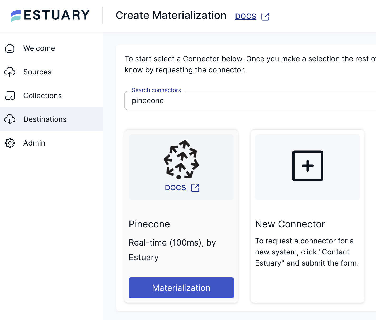
5. Navigate to the "Destinations" section.
6. Click on "Create New Materialization".
7. Choose "Pinecone" as your materialization connector.

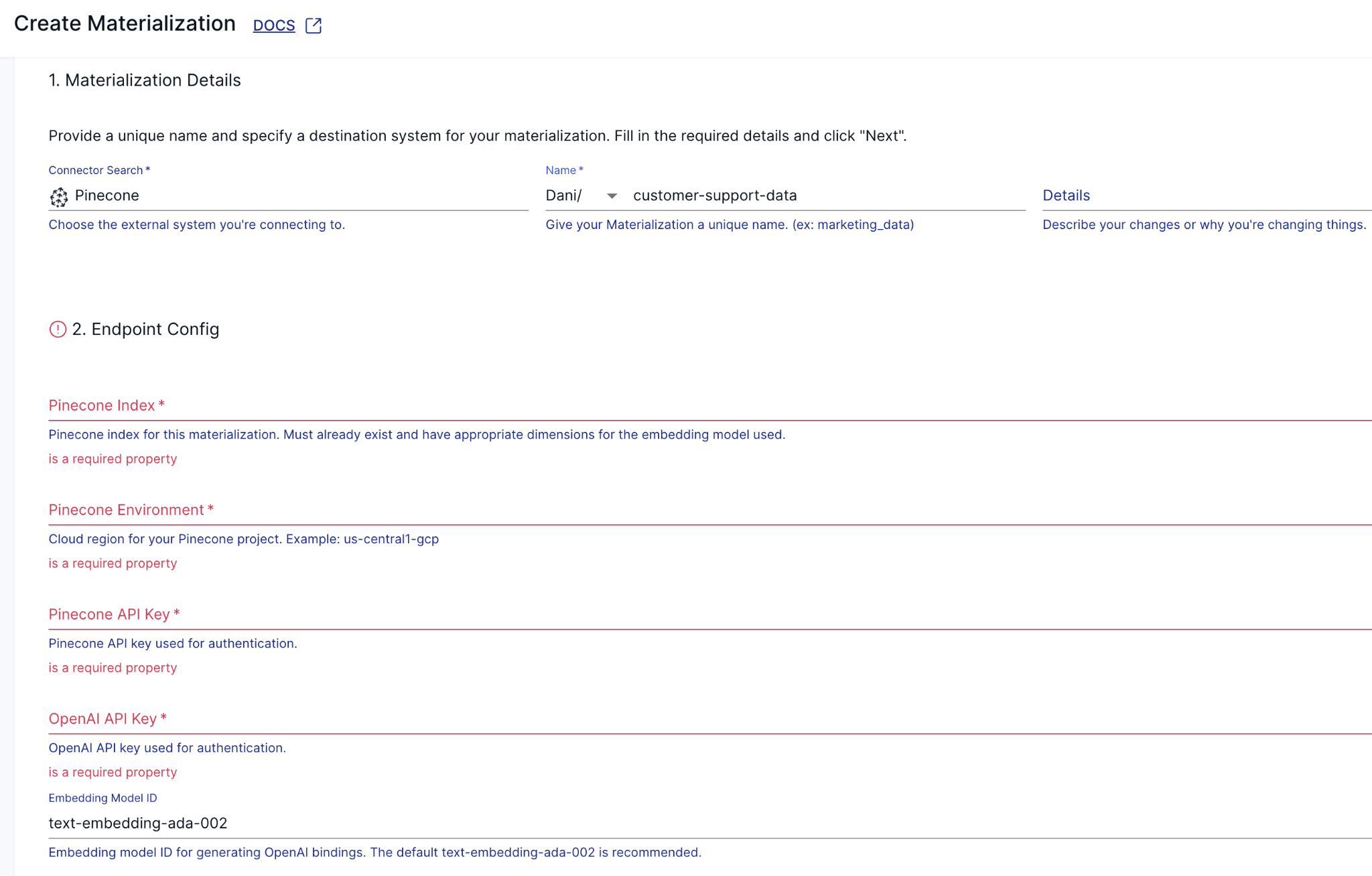
Next, configure the Materialization. Enter all the configuration details required by the connector; such as your Pinecone index name, environment identifier, and both API keys.

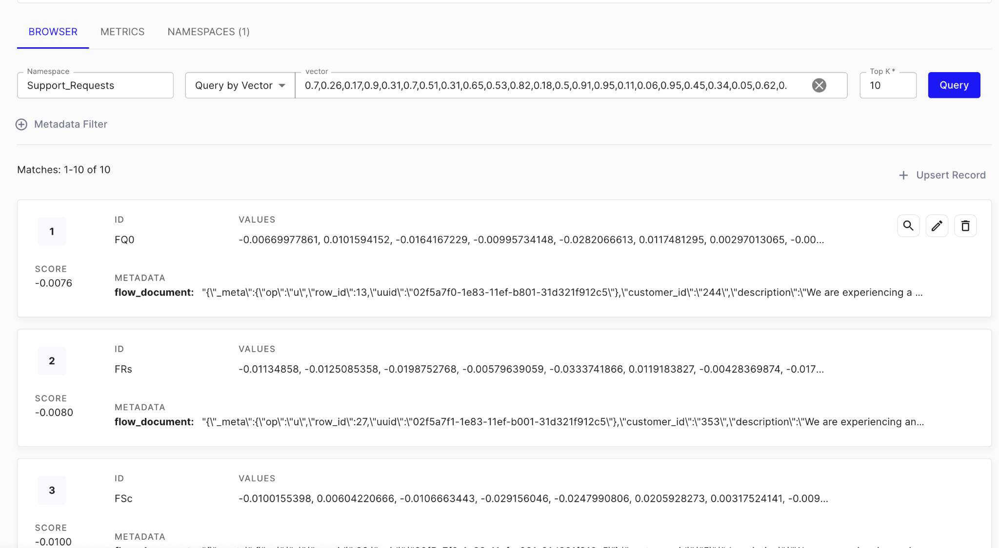
Finally, Save & Publish the Materialization. To verify that it’s working correctly, you can head over to the Pinecone web UI and make sure there are embeddings in the index. 

It should look something like this:

The Pinecone materialization connector creates a vector embedding for each document in the collection generated by the source connector, along with additional metadata. The structure of the embeddings is straightforward: the entire document, along with the metadata fields produced during capture from the source, is packaged under the "flow_document" key. These metadata fields include a UUID value, the original row ID, and the operation type that triggered the change event.

Pinecone supports upserts, allowing you to use only the latest version for each record, which is important for avoiding stale data.

Step 4. It’s RAG time!

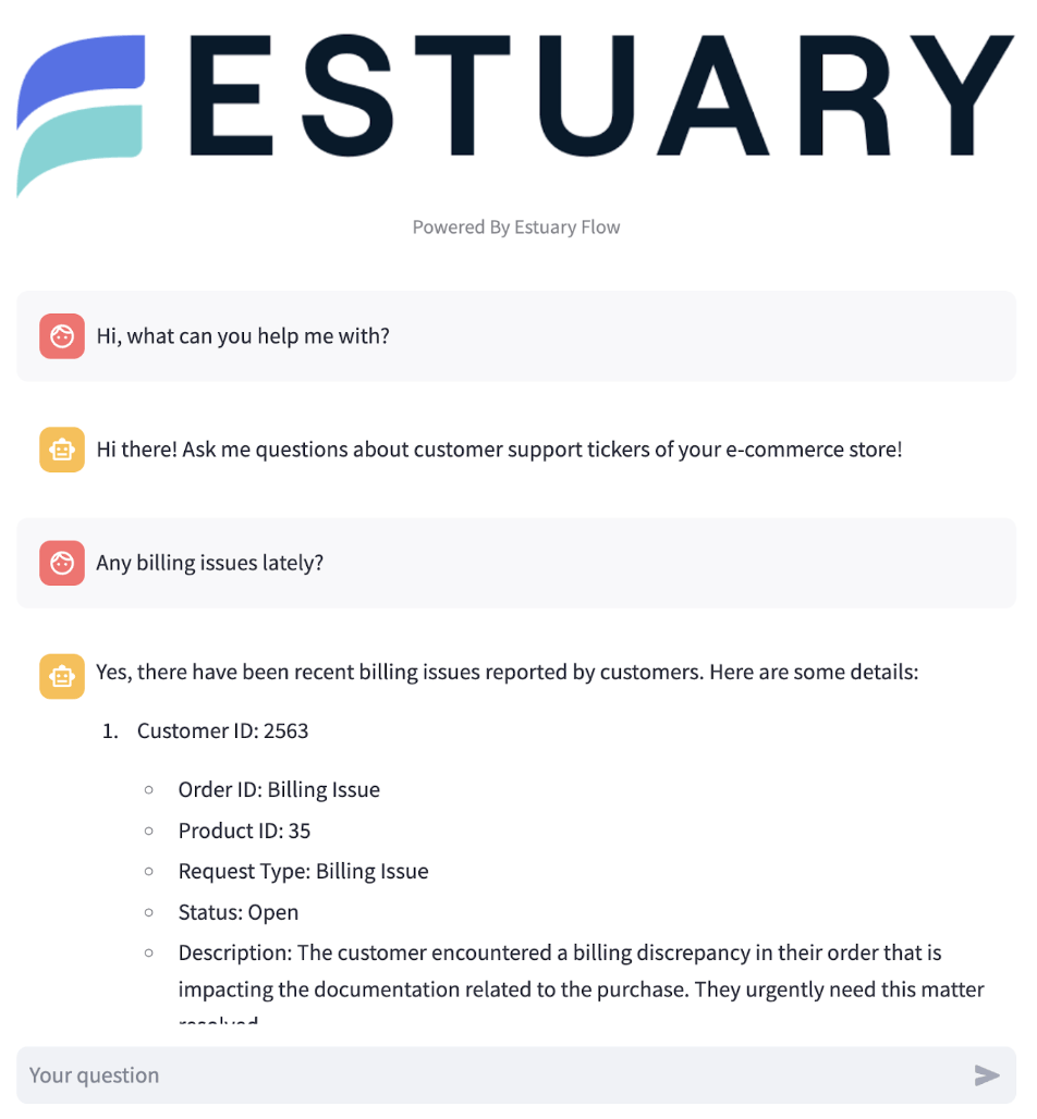
Now that you have a steady flow of incoming data and embeddings are being generated incrementally, as the last step, spin up the Streamlit chat application so you’ll have a familiar interface that allows you to access the customer support tickets.

plaintext
docker compose up streamlit

Navigate to http://localhost:8502 and try asking a few questions!

When data is added to the Snowflake, it is immediately converted into vectors and stored in Pinecone. This quick processing allows the chat application to include the data without any delays, which is especially crucial for time-sensitive data.

When you submit a question to the Streamlit application, it undergoes vectorization using the same embedding model as the Pinecone Materialization connector. This enables a similarity search to be carried out against the existing vectors in the space.

The application identifies the top 5 most semantically similar vectors, which are vectorized versions of the documents originating from Snowflake. It then composes a prompt for submission to OpenAI’s API, which utilizes a large language model to format the data as if a human were responding.

Wrapping up

By combining Snowflake, Estuary Flow, and Pinecone, you learned how to build a real-time incremental vector embedding generation pipeline coupled with a Streamlit chat application that completes an end-to-end RAG project.

We hope this tutorial has provided you with the knowledge and tools to implement your data flows and leverage the full potential of Estuary Flow and LLMs in your data products.

If you want to learn more, make sure you read through the Estuary documentation.

You’ll find instructions on how to use other connectors here. You can connect to just about any source, not just Snowflake! There are more tutorials here. 

Also, don’t forget to join the Estuary Slack Community!