Introduction
When dealing with real-time data—whether from IoT sensors, financial market feeds, or APIs—swift processing is essential for companies to take proactive measures with sudden changes within the data. Applications range from fraud detection and stock market trading to system monitoring, allowing teams to address issues immediately when anomalies are detected. Real-time data becomes particularly valuable when it delivers actionable insights into abnormal patterns, enabling users to forecast changes and make informed decisions.
In this article, I'll walk through an example of real-time data ingestion, where I'll feed 5 day forecast weather data from the OpenWeather API into MongoDB and process the data into Databricks and perform real time analytics. By monitoring trends in weather data—such as temperature, humidity, and wind patterns—on the East Coast cities of the U.S., we'll use Databricks to detect anomalies. We'll also create visualizations of these weather patterns, allowing users to understand weather disruptions more effectively.
Using Estuary, we can set up a real-time data integration pipeline between MongoDB and Databricks in just a few minutes.
Pre-requisites
- MongoDB: Configure a MongoDB instance to store incoming weather data.
- Databricks Account: Set up a free or premium Databricks workspace.
- Azure (or AWS) Account (Optional): To connect Databricks to ADLS2 for storing Unity Catalog tables.
- Estuary Account: Visit the Estuary website and sign up for the free tier or initiate a 30-day trial on the paid tier.
- VS Code (or any preferred IDE): For ingesting API data into MongoDB collections.
- OpenWeatherMap API Key: To access the weather forecast data (5-day forecast).
Real Time API Data Ingestion to Databricks Overview
Here's how it works:
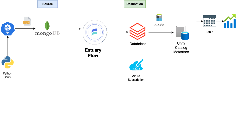
- Retrieve API Data into MongoDB: Use a Python script to call the OpenWeather API and ingest the data into your MongoDB collections.
- Setup MongoDB Change Streams: Use MongoDB change streams to listen for new documents (i.e., new city weather data) being added. Change streams allow real-time notifications, which will be helpful to send data to Databricks without polling MongoDB continuously.
- Set up MongoDB as a Source Connector with Estuary: Configure real-time ingestion from MongoDB by creating a new capture in Estuary, using your MongoDB endpoint credentials.
- Create Azure Account and Resources: Create an Azure account (or another cloud provider such as AWS/GCP) and provision two resources: Databricks and ADLS2 (Azure Data Lake Storage 2), and make sure they have the proper user roles. Ensure Databricks is set up with a premium account, as you will store data in the Unity Catalog Metastore.
- Add Databricks as a Destination in Estuary for Materialization: After configuring your Databricks account and Unity Catalog, create a materialization of the MongoDB source. Set Databricks as the destination to migrate the source data into the Unity Catalog.
- Perform Real-Time Analytics on the Data: Once the table is loaded into the Unity Catalog, leverage SQL Warehouse to query the data or create a notebook for in-depth analysis. This may involve detecting patterns and anomalies in the weather data using machine learning libraries, as well as crafting insightful visualizations to better understand the data.
Overview of MongoDB: The Data Source
MongoDB is a NoSQL database that stores data in flexible, JSON-like documents, known as BSON (Binary JSON), rather than in traditional tabular relations (rows and columns). This allows for dynamic schema design, which means data structures can evolve over time without requiring changes to existing schemas. MongoDB is widely known for its scalability, flexibility, and performance.
Why MongoDB is Useful for API Data or Real-Time Ingestion
- Flexible Schema: MongoDB's document-oriented structure allows for storing complex and unstructured data (like API responses) without needing to define a fixed schema in advance.
- Scalability: MongoDB excels at handling large volumes of data across distributed clusters. For real-time API data ingestion, MongoDB’s horizontal scaling makes it easy to distribute data across multiple nodes for performance optimization.
- Real-Time Ingestion and Change Streams: MongoDB supports change streams, which allow you to react in real time to changes in your database. This is particularly useful for real-time data ingestion, where updates or changes to incoming data (e.g., weather data updates) can be tracked and processed without polling the database repeatedly.
Overview of Databricks
Databricks is a cloud-based data engineering and analytics platform built on Apache Spark, designed to unify data science, data engineering, and business analytics. It provides a collaborative environment for teams to build and deploy machine learning models, process massive datasets, and perform real-time analytics. Databricks is available on major cloud platforms such as AWS, Azure, and Google Cloud, and it provides a scalable solution to handle large volumes of data.
Key Features of Databricks:
- Delta Lake: Databricks offers Delta Lake, a storage layer that boosts data lakes' performance and reliability. It adds ACID transactions, data versioning, and scalable metadata handling, making data management more robust and analytics-friendly.
- Real-Time Streaming: Databricks supports structured streaming, enabling real-time data ingestion, processing, and analytics. This feature is crucial for applications like real-time API integrations.
- ML flow Integration: Databricks seamlessly integrates with MLflow, simplifying machine learning model management. This includes experiment tracking, model deployment, and lifecycle management.
- Unity Catalog: Unity Catalog serves as Databricks' unified governance solution. It provides centralized governance and granular access control over all data assets within the platform. By ensuring data lineage across various sources, it streamlines management of data from diverse locations such as cloud data lakes or MongoDB.
Setting up MongoDB
- Collect Weather Forecast API Data : Use the OpenWeatherMap 5-Day Forecast API to retrieve weather forecast data for any location worldwide. The forecast includes data in 3-hour intervals. Be sure to call this API and securely store the API key for future requests.
- Create a MongoDB Atlas cluster: This tutorial uses Atlas as the source database, where you will ingest OpenWeatherMap 5-Day Forecast API, with database as weather_db, and collection name as weather_forecast.
- Fetch Weather Data using a Python Script in your IDE: Fetch weather data for multiple cities from the OpenWeatherMap API, where you combine the cities in the East Coasts’ 3 hour forecasts into a single JSON file, and then insert this combined data into a MongoDB collection.
python# Replace with your API key
API_KEY = "YOUR_API_KEY"
# MongoDB connection details
username = 'YOUR_USERNAME'
db_password = 'YOUR_DB_PASSWORD'
cluster_name='YOUR_CLUSTER'
uri = f"mongodb+srv://{username}:{db_password}@{cluster_name}.mongodb.net/?retryWrites= true&w=majority&appName={cluster_name}"
DB_NAME = "weather_db" # Database name
COLLECTION_NAME = "weather_forecast" # Collection name
# OpenWeatherMap API credentials
cities = ["Portland", "Boston", "New York", "Philadelphia", "Baltimore", "Washington", "Richmond", "Jacksonville", "Miami", "Savannah"]
def flatten_weather_data(combined_weather_data):
 flattened_data = []

 for city_entry in combined_weather_data:
 city_info = city_entry['city']
 for forecast in city_entry['forecasts']:
 forecast_details = forecast['forecast']['details']

 # Create a flattened entry for each forecast
 flattened_entry = {
 "city_id": city_info.get('id'),
 "city": city_info.get('name'),
 "country": city_info.get('country'),
 "latitude": city_info.get('latitude'),
 "longitude": city_info.get('longitude'),
 "forecast_time": forecast['forecast']['time'],
 "temp": forecast_details['main']['temp'],
 "feels_like": forecast_details['main'].get('feels_like'),  "temp_min": forecast_details['main'].get('temp_min'),  "temp_max": forecast_details['main'].get('temp_max'),  "pressure": forecast_details['main'].get('pressure'),  "sea_level": forecast_details['main'].get('sea_level'),  "ground_level_pressure": forecast_details['main'].get('grnd_level'),  "humidity": forecast_details['main'].get('humidity'),  "weather": forecast_details['weather'][0].get('description') if forecas t_details.get('weather') else None,
 "wind_degree": forecast_details['wind'].get('deg'),  "wind_speed": forecast_details['wind'].get('speed'),  "wind_gust": forecast_details['wind'].get('gust', None),  "cloud_coverage": forecast_details['clouds'].get('all'),  "visibility": forecast_details.get('visibility', None)  }
 flattened_data.append(flattened_entry)

 return flattened_data
def fetch_weather_data():
 # Initialize an empty list to store weather data for all cities  multiple_cities_weather_data = []

 for city in cities:
try:
# Construct API URL
 URL = f"https://api.openweathermap.org/data/2.5/forecast?q={city}&appid={AP I_KEY}"
 response = requests.get(URL)
 response.raise_for_status() # Raise an error for bad responses (4xx and 5x x)
 		weather_data = response.json()

 # Extract city information
 city_info = weather_data.get('city', {})
 city_data = {
 "id": city_info.get('id'),
 "name": city_info.get('name'),
 "latitude": city_info.get('coord', {}).get('lat'),  "longitude": city_info.get('coord', {}).get('lon'),  "country": city_info.get('country'),
 "population": city_info.get('population'),
 "timezone": city_info.get('timezone'),
 }

 # Collect all forecasts for this city
 city_forecasts = []
 for forecast in weather_data['list']:
 # Convert Unix timestamp to readable datetime
 forecast_time = datetime.fromtimestamp(forecast['dt'], tz=timezone.ut c).strftime('%Y-%m-%d %H:%M:%S')

 # Construct the data to insert
 forecast_with_city = {
 "city": city_data,
 "forecast": {
 "time": forecast_time,
"details": forecast
 }
 }
 city_forecasts.append(forecast_with_city)

 # Add city forecasts to combined_weather_data
 multiple_cities_weather_data.append({
 "city": city_data,
 "forecasts": city_forecasts
 })

 print(f"Fetched and processed weather data for {city}")

 except requests.exceptions.RequestException as e:
 print(f"Error fetching weather data for {city}: {e}")
 except Exception as e:
 	print(f"An error occurred for {city}: {e}")
 # Insert each city's weather data into MongoDB individually
 try:
 client = MongoClient(uri)
 db = client[DB_NAME] # Create or connect to the database
 collection = db[COLLECTION_NAME] # Create or connect to the collection
# Flatten and insert the data
flattened_weather_data = flatten_weather_data(multiple_cities_weather_data)  collection.insert_many(flattened_weather_data)
 client.close()

print("Combined weather data successfully inserted into MongoDB!")
 except PyMongoError as e:
 	print(f"Error inserting data into MongoDB: {e}")
# Call the function to fetch and combine weather data
fetch_weather_data()
API_KEY : Replace "YOUR_API_KEY" with your actual API key.
username : Replace 'YOUR_USERNAME' with your MongoDB username.
db_password : Replace 'YOUR_DB_PASSWORD' with your MongoDB password.
uri : Update the MongoDB connection string with your actual cluster details.
This code retrieves weather forecast data for a list of cities using the OpenWeatherMap API, processes it, and then stores a flattened version of this data into the weather_forecast collection in MongoDB, making each forecast an individual document.
3. Apply MongoDB’s Change Stream to check for updates in the Weather API, and runs if it detects new forecasts.
python# Function to check for changes in MongoDB using change streams
def check_for_changes():
 	client = MongoClient(uri)
 	db = client[DB_NAME]
 	collection = db[COLLECTION_NAME]
 try:
 	# Listen for changes in the weather_forecast collection
 	with collection.watch(max_await_time_ms=5000) as stream: # Wait for 5  seconds max  print("Checking for changes...")
 for change in stream:
 	print(f"Change detected: {change}")
 if change['operationType'] == 'insert':
 	print(f"New forecast inserted: {change['fullDocument']}")     return True # Stop listening once a change is detected  except PyMongoError as e:
 	print(f"MongoDB change stream error: {e}")
 	return False
 finally:
 	client.close()
 # If no changes detected within the timeout period, return False
 return False
check_for_changes()
The check_for_changes function monitors a MongoDB collection ( weather_forecast ) for new changes, specifically focusing on detecting new data entries. It uses MongoDB’s change streams feature, which allows real-time notifications of data changes in the database.
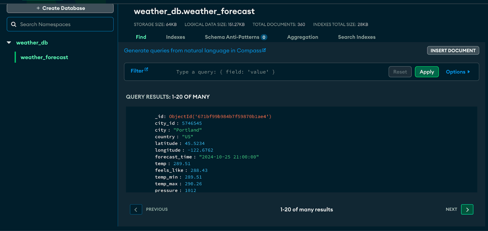
After running the python script, you get the following output:
- weather_db is the Database Name, weather_forecast is the collection name.
Load Data From MongoDB to Databricks using Estuary
By integrating MongoDB and Databricks through tools like Estuary, you can create a seamless data pipeline. MongoDB can handle the real-time API data ingestion, while Databricks can perform the advanced analytics and reporting—ensuring high performance and real-time insights for decision-making.
In Databricks, we can extract useful features like temperature change rate, wind gust spikes, or moving averages of weather metrics to give more context for anomaly detection. We can utilize statistical methods and Anomaly Detection Techniques such as Z-Score/Threshold-Based Approach or Machine Learning-Based Approaches to detect anomalies and create visualization dashboards.
Benefits of Using Estuary
Estuary is a unified data integration platform that's built from the ground up for the cloud and handles both streaming and batch data flows.
Real-Time Data Synchronization with CDC
- Immediate Business Insights: Estuary’s Change Data Capture (CDC) technology ensures that any changes in MongoDB data are reflected in Databricks within seconds. MongoDB’s Change Streams provide real-time monitoring of data modifications, enabling Estuary to subscribe to detailed change events such as insertions, updates, or deletions. This ensures efficient data propagation from MongoDB to Databricks, allowing for immediate analysis and informed decision-making based on the most current data.
- Effortless Data Integration: Estuary’s automated pipelines eliminate the need for manual coding, allowing data practitioners to set up and manage integrations between MongoDB and Databricks effortlessly.
- Enterprise-ready: Estuary can be deployed in any enterprise networking environment using Private Deployments.
- Managed Backfills: Managed backfills allow you to fill your destination storage with the historical data of a source system. With Estuary, you can easily handle and orchestrate these historical backfills without breaking your real-time streaming ingestions.
Configure MongoDB as a Source to Estuary
- Sign in to your Estuary account or sign up for free.
- Select Sources from the side menu. Then, click on the + NEW CAPTURE button on the Sources page.
- Search for MongoDB using the Source connectors field on the Create Capture page. When the connector appears in search results, click its Capture button.
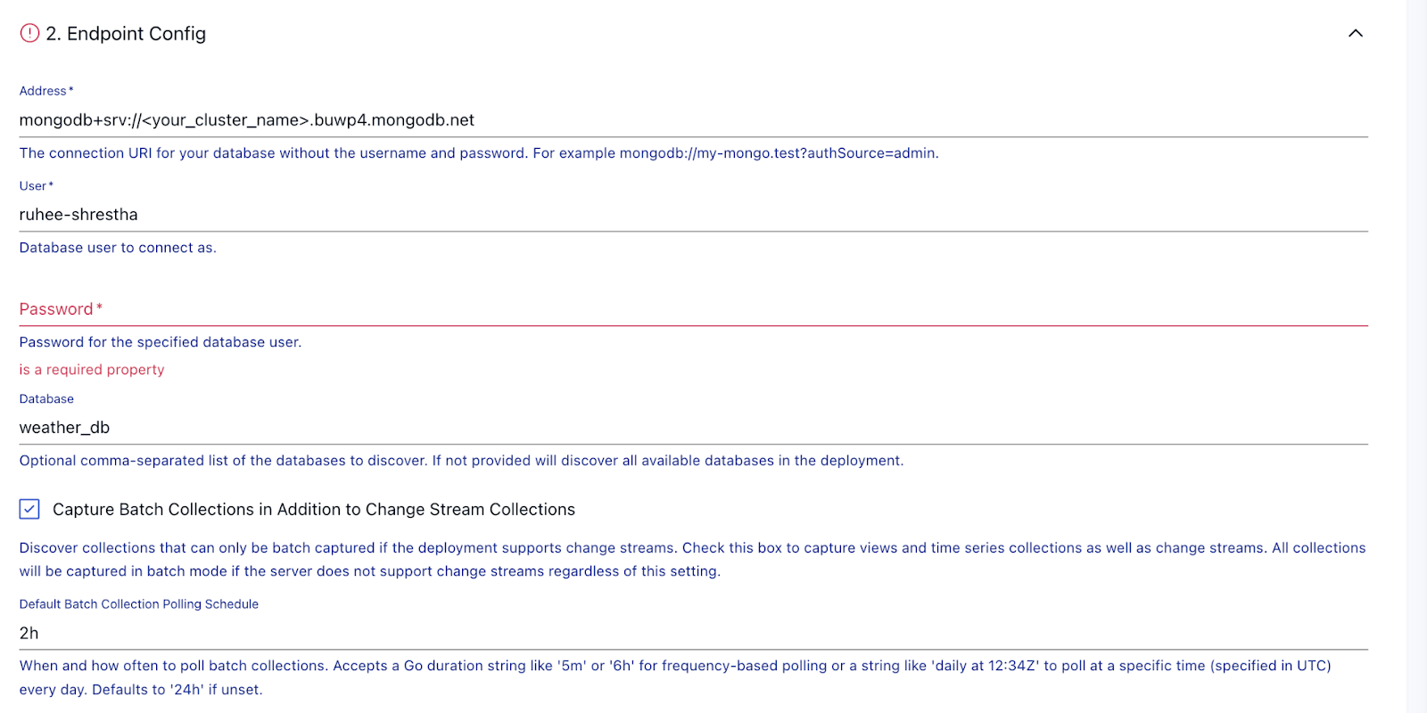
You'll be redirected to the connector configuration page, where you can specify the following details:
- Name: Enter a unique name for your source capture.
- User: Provide the username of the user.
- Password: Provide the Password of the user.
- Address: Provide a connection URI (Uniform Resource Identifier) for your database
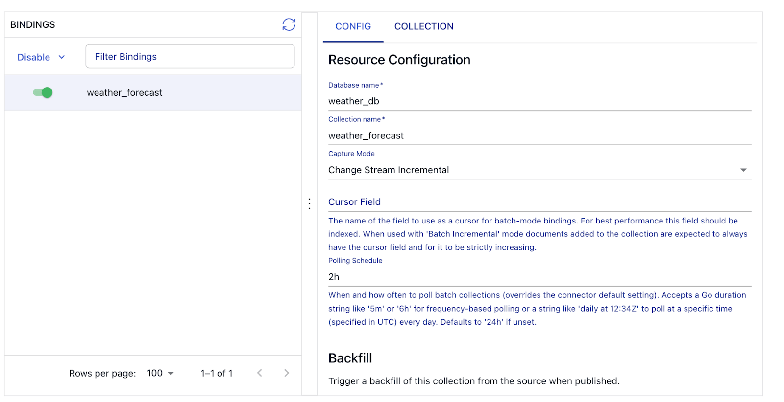
plaintextmongodb+srv://<cluster_name>.buwp4.mongodb.net After you press the blue “Next” button in the top right corner, Estuary will automatically crawl through the connection to discover available resources. Next up, you’ll see the third, and final configuration section, where you are able to view and choose from all the databases and collections which are discovered by Estuary.
- Click on NEXT. Then click on SAVE AND PUBLISH.
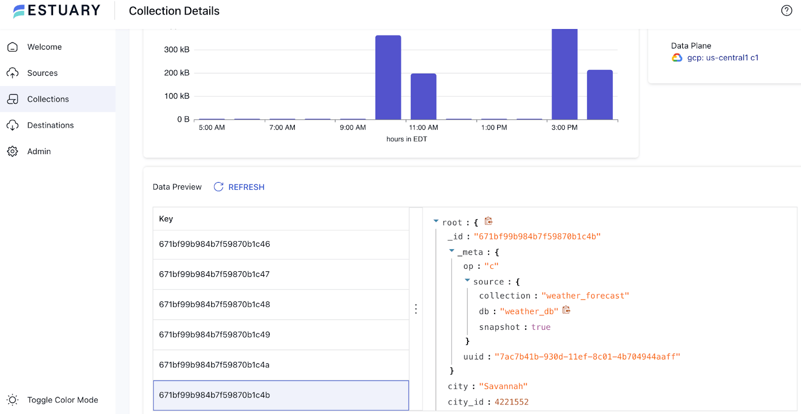
After you insert the document, check out your Collections Page, and Data preview on the Estuary UI to verify it has arrived.
The next step is to set up our materialization (destination).
Setting up Databricks
- Create a Databricks Resource in your Azure Account, and make sure it is a Premium account which supports Unity Catalog.
- Make sure your workspace has Unity Catalog enabled. Next steps if your workspace is not enabled for Unity Catalog.
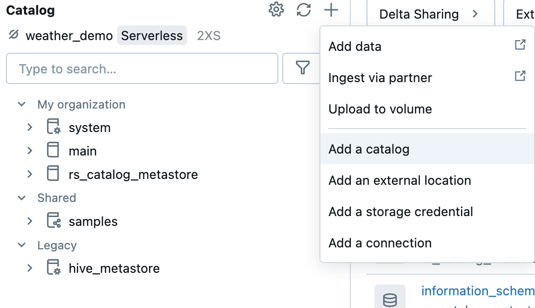
3. Create a Unity Catalog by :
a. Go to Catalog → + → Add a catalog
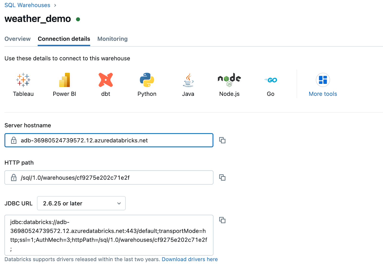
4. Create a SQL Data Warehouse, called ‘weather_demo’ and save the data warehouse details, such as the http path and server host name.
Store the following credentials from Databricks to be used for creating materialization:
- URL: https://adb-xxxxxxxxxxxxxx.azuredatabricks.net
- Unity Catalog: rs_catalog_metastore
- HTTP path: /sq/1.0/warehouses/xxxxxxxxx
Configure Databricks as the Destination - Estuary
- Select Destinations from the dashboard side menu. On the Destinations page, click on + NEW MATERIALIZATION.
- Search for Databricks in the Search connectors field on the Create Materialization page. When the connector appears, click on its Materialization button.
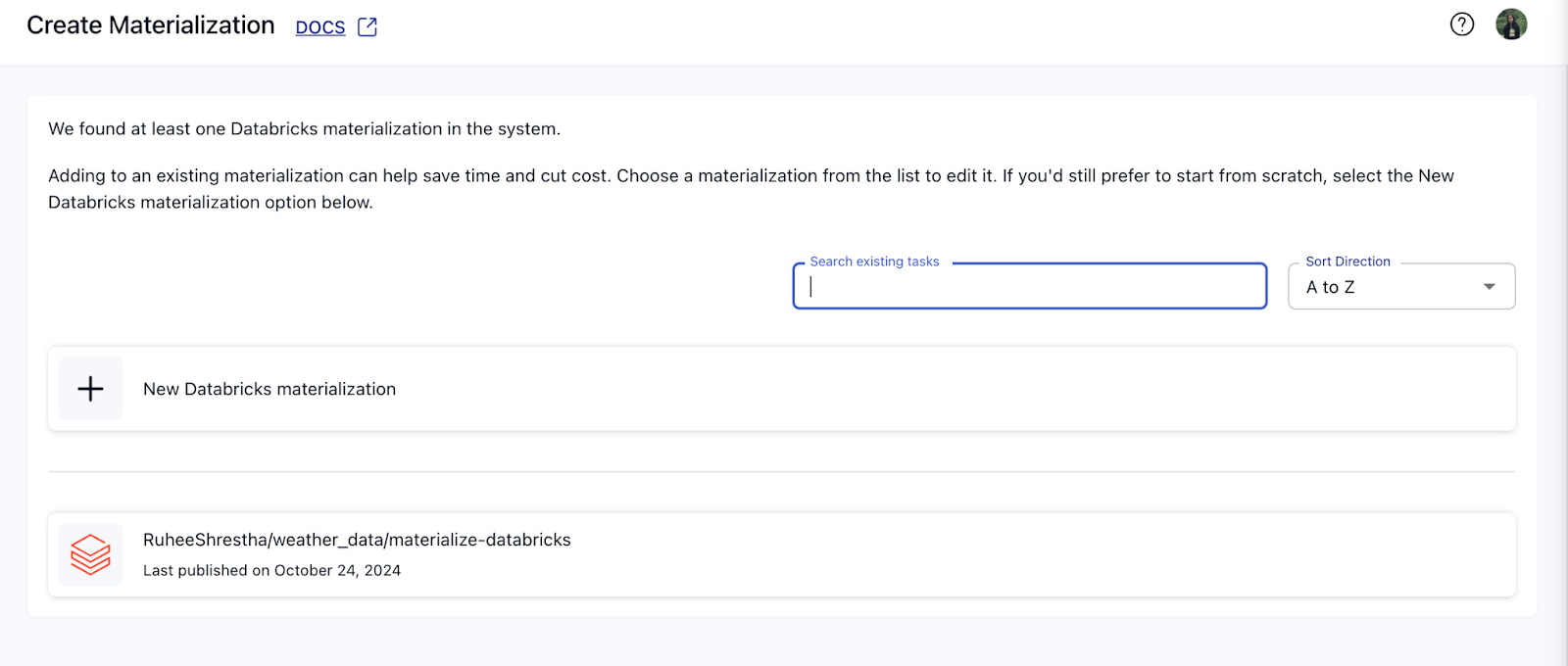
Pictured above, I have already created a databricks materialization, so I can go ahead and select that one to update the weather data.
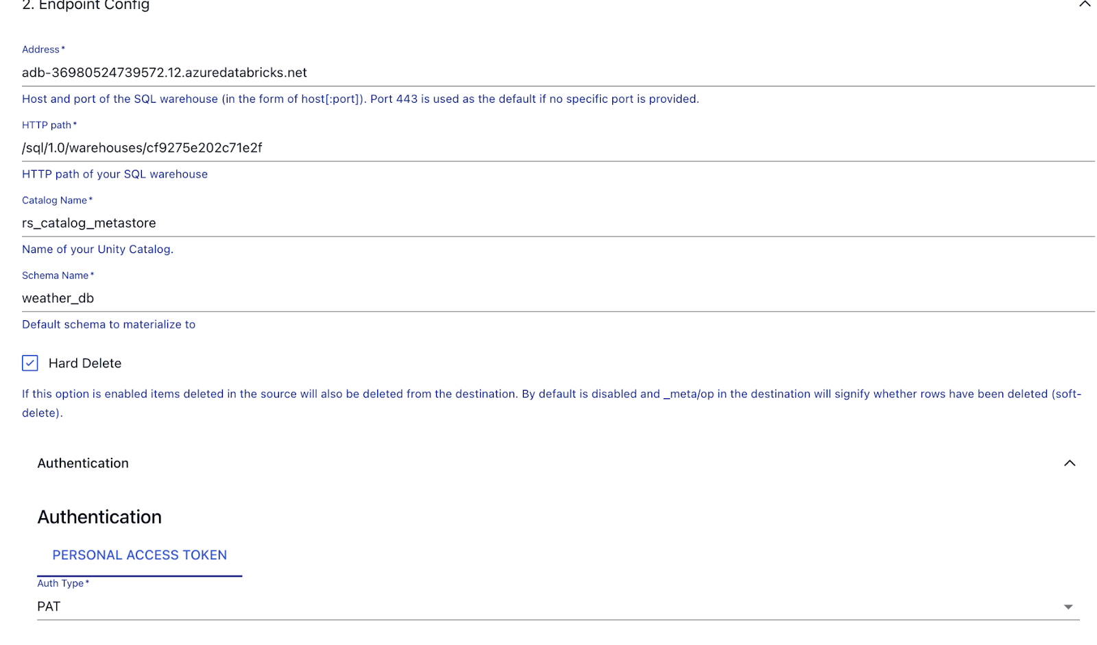
c. Setting up Endpoint Config
- Name: Enter a unique name for your materialization.
- Address: Provide Databrick’s host and port name.
- HTTP Path: Enter the HTTP path for your SQL warehouse.
- Unity Catalog Name: Specify the name of your Databricks Unity Catalog.
- Personal Access Token: Provide a Personal Access Token which has permissions to access the SQL warehouse.
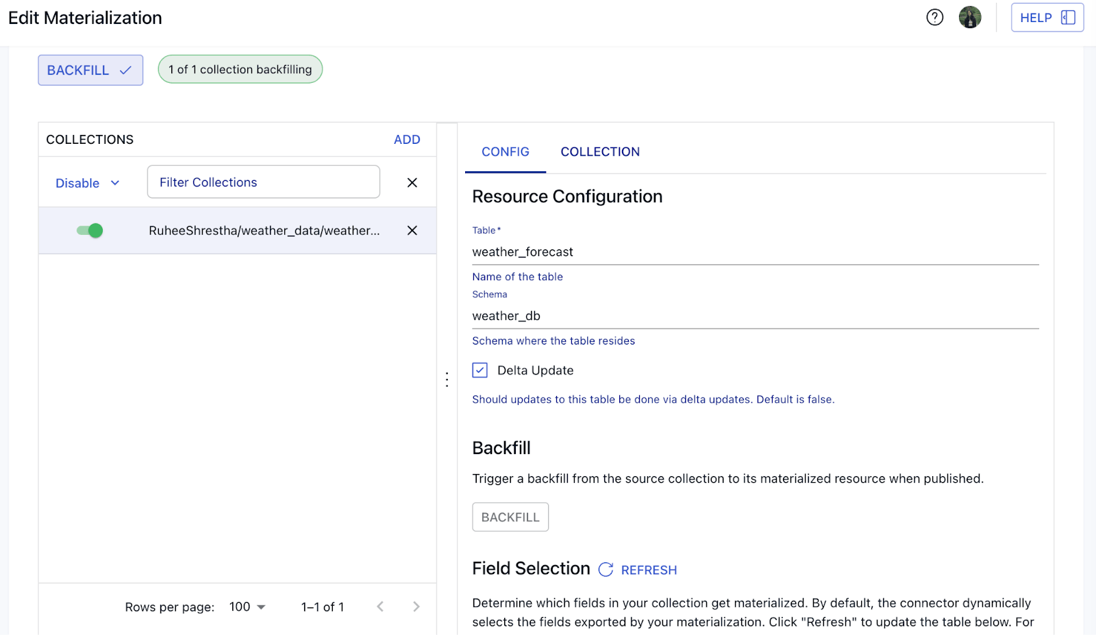
D. Create Source Collections
E. Click on NEXT and then select the specific collections that you want ingested into Databricks f. Click on SAVE AND PUBLISH to complete the configuration process.
The real-time connector will materialize the data ingested from the Estuary collection of MongoDB data into the Databricks destination.
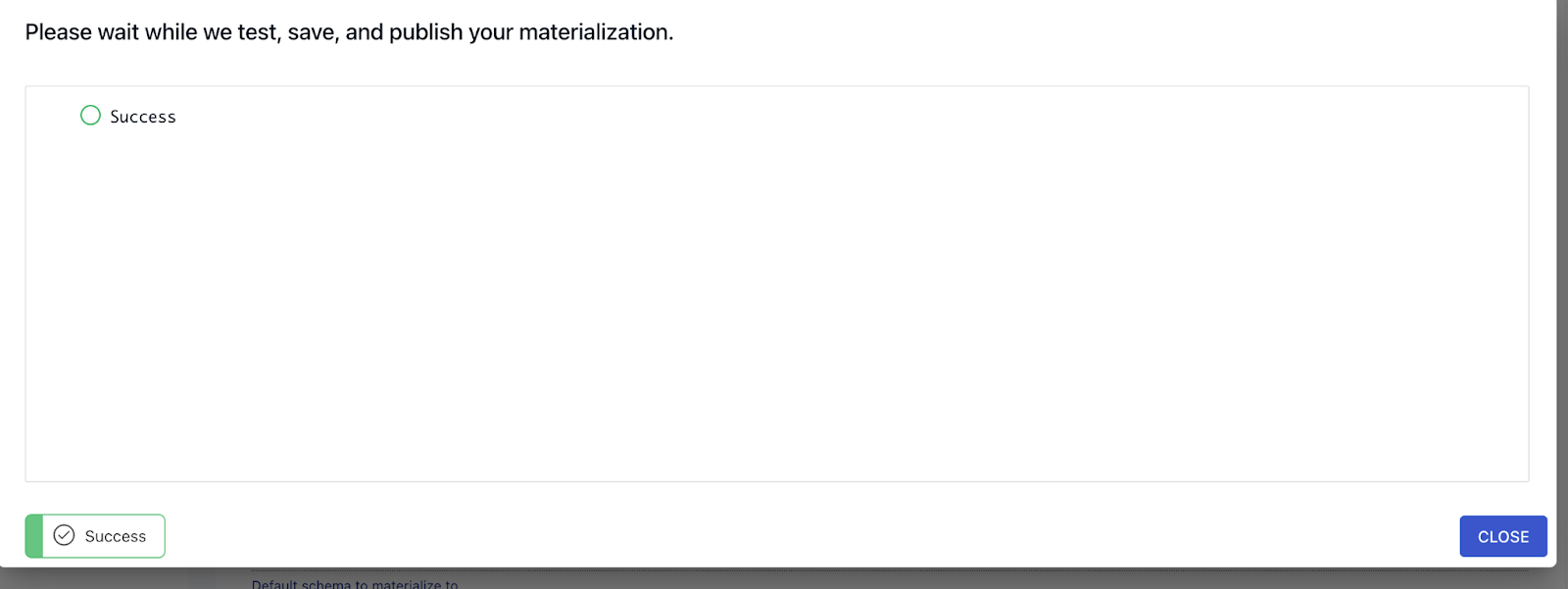
Output:
In your Destinations page, now you will see that the data has been written into Databricks successfully indicated by the green button.
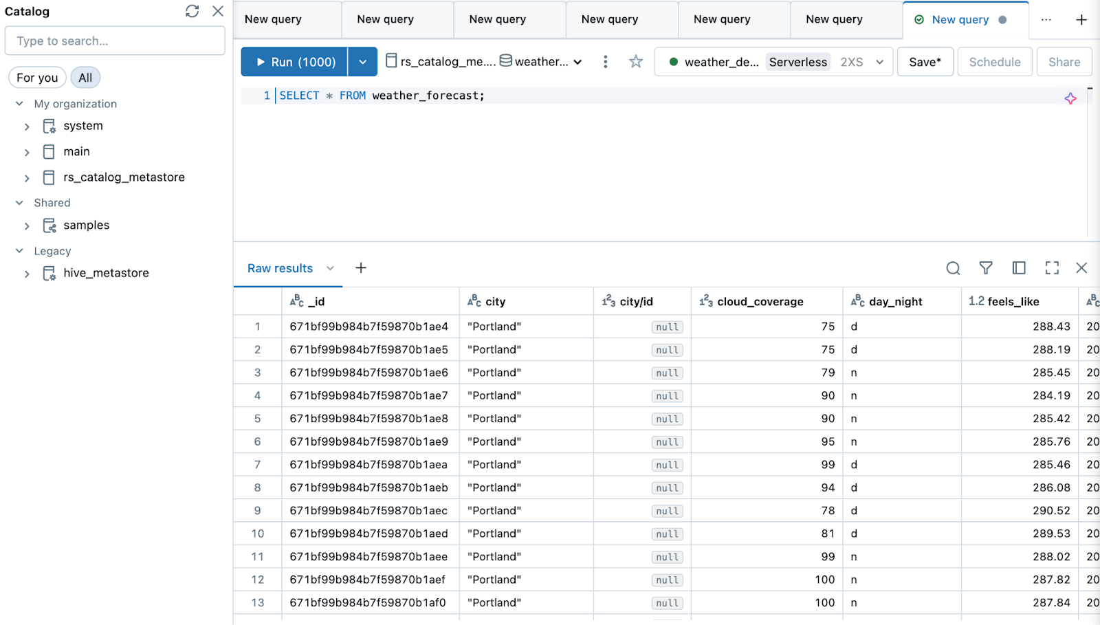
You can start querying the data using SQL warehouse or you can view the data on your notebook to start cleaning the data, and performing analytics.
Performing Analytics in Databricks
- Read the Table from Catalog
plaintextweather_df = spark.sql("select * from rs_catalog_metastore.weather_db.weather_forecast") display(weather_df) Output:
| _id | city | cloud_coverage | day_night | feels_like | forecast_time | humidity | pop | pressure | sea_level | temp | temp_max | temp_min | visibility |
| 671bf99b984b7f59870b1ae4 | "Portland" | 75 | d | 288.43 | 2024-10-25 21:00:00 | 47 | 0 | 1012 | 1012 | 289.51 | 290.26 | 289.51 | 10000 |
| 671bf99b984b7f59870b1ae5 | "Portland" | 75 | d | 288.19 | 2024-10-26 0:00:00 | 42 | 0 | 1011 | 1011 | 289.41 | 289.41 | 289.2 | 10000 |
| 671bf99b984b7f59870b1ae6 | "Portland" | 79 | n | 285.45 | 2024-10-26 3:00:00 | 43 | 0 | 1011 | 1011 | 286.9 | 286.9 | 285.6 | 10000 |
| 671bf99b984b7f59870b1ae7 | "Portland" | 90 | n | 284.19 | 2024-10-26 6:00:00 | 44 | 0 | 1013 | 1013 | 285.73 | 285.73 | 285.73 | 10000 |
| 671bf99b984b7f59870b1ae8 | "Portland" | 90 | n | 285.42 | 2024-10-26 9:00:00 | 48 | 0 | 1015 | 1015 | 286.75 | 286.75 | 286.75 | 10000 |
| 671bf99b984b7f59870b1ae9 | "Portland" | 95 | n | 285.76 | 2024-10-26 12:00:00 | 81 | 1 | 1016 | 1016 | 286.28 | 286.28 | 286.28 | 10000 |
Trends in weather by city:
plaintextaverage_by_city = weather_df.groupBy("city").agg(
 F.avg("humidity").alias("avg_humidity"),
 F.avg("temp_in_c").alias("avg_temp_in_c"),
 F.avg("wind_speed").alias("avg_wind_speed"),
 F.avg("pressure").alias("avg_pressure")
)
display(average_by_city)
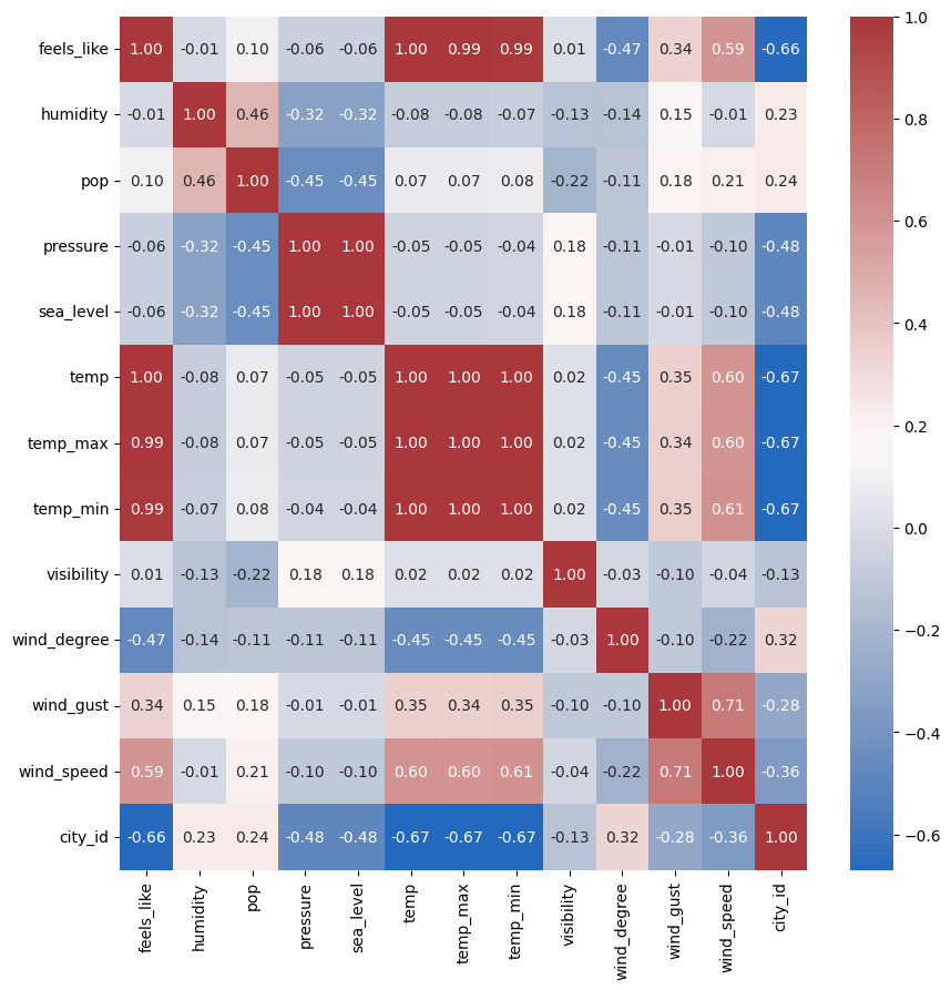
Multivariate Analysis
plaintext# plot heatmap to show correlation between the 16 numerical features
import matplotlib.pyplot as plt
import seaborn as sns
import pandas as pd
df = weather_df.toPandas()
# plot heatmap to show correlation between the 16 numerical features plt.figure(figsize=(10, 10))
corr = df.iloc[:, 3:20].corr()
sns.heatmap(corr, annot=True, cmap = 'vlag', fmt=".2f")
plt.show() Anomaly Detection Methods
Temperature Deviation Threshold - Rolling Mean
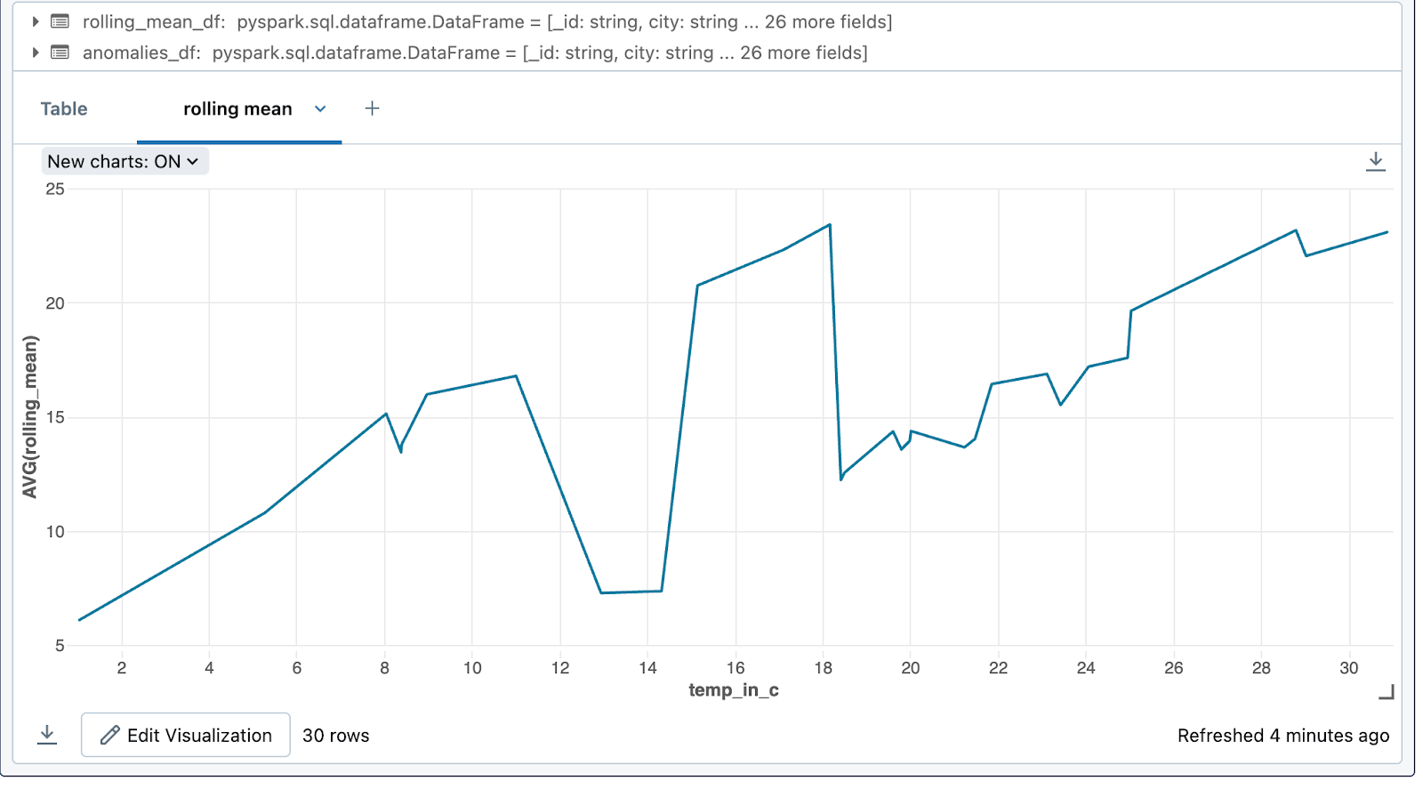
We can calculate a rolling mean over recent updates (e.g., a 24-hour period) and flag anomalies when the current temperature deviates from this mean by a certain threshold (e.g., ±5°C).
plaintextfrom pyspark.sql import Window
from pyspark.sql.functions import avg, col, abs
# Define a window for a rolling 24-hour period (8 rows per city sorted by forecast_time)
window_spec = Window.partitionBy("city").orderBy("forecast_time").rowsBetween(-7, 0)
# Calculate rolling mean and temperature deviation from it
rolling_mean_df = weather_df.withColumn("rolling_mean", avg("temp_in_c").over(window_spec)) \
    .withColumn("temp_deviation", abs(col("temp_in_c") - col("rolling_mean"))) \
    .withColumn("is_anomaly", (col("temp_deviation") > 5))
anomalies_df = rolling_mean_df.filter(col("is_anomaly") == True)
display(anomalies_df.select("city", "forecast_time", "temp_in_c", "temp_deviation", "rolling_mean", "is_anomaly"))
Create a Line Chart: Visualize the Temperature and rolling_mean over time for each city to observe deviations.
Anomaly Detection by Rolling Mean - Temperature (in C)
Anomaly Detection by Rolling Mean - Humidity
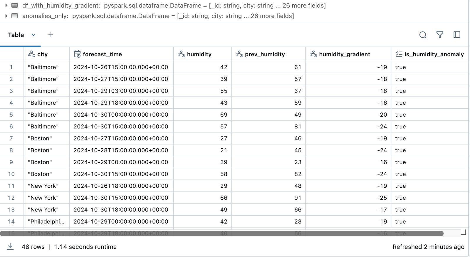
To identify anomalies in humidity that vary consistently over time, you can apply a similar approach as you did for temperature. Here's how you can calculate the relative humidity fluctuations between consecutive updates and flag anomalies based on a specified threshold (e.g., ±15% relative humidity) in PySpark.
Here’s how you can implement this:
plaintextfrom pyspark.sql import Window
from pyspark.sql.functions import col, lag, abs
# Define a window partitioned by city and ordered by forecast_time
window_spec_humidity = Window.partitionBy("city").orderBy("forecast_time")
# Assuming 'Humidity' is a column in your DataFrame
df_with_humidity_gradient = weather_df.withColumn("prev_humidity", lag("humidity").over(wi ndow_spec_humidity))
# Calculate the humidity gradient (rate of change)
df_with_humidity_gradient = df_with_humidity_gradient.withColumn(
 "humidity_gradient",
 col("humidity") - col("prev_humidity")
)
# Flag anomalies based on the threshold (±15%)
humidity_threshold = 15
df_with_humidity_gradient = df_with_humidity_gradient.withColumn(
 "is_humidity_anomaly",
 abs(col("humidity_gradient")) > humidity_threshold
)
anomalies_only = df_with_humidity_gradient.filter(col("is_humidity_anomaly") == True)
# Show the results
display(anomalies_only.select(
 "city", "forecast_time", "humidity", "prev_humidity",
 "humidity_gradient", "is_humidity_anomaly"
))
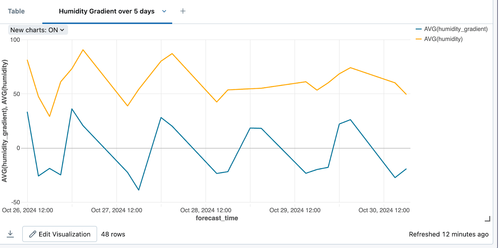
Visualizing Humidity Anomalies
This setup allows you to visualize how the humidity values change over time alongside the rate of change, providing insights into any significant fluctuations or anomalies.
Anomaly Detection Method using ML : k-NN
The k-Nearest Neighbors algorithm, (k-NN) is a supervised machine learning algorithm that is widely used to solve classification problems. k-NN algorithm assumes that similar things exist in close proximity.
We applied this algorithm to the dataset as follows:
- We normalized the temperature values to ensure uniform scaling.
- We applied the k-NN algorithm to identify anomalies in the temperature data.
- We selected the optimal k value to achieve the maximum accuracy of the model. The common case is k = 5. So, in the example, we initiated that k = 5 and proceeded with the process.
- We calculated z-scores for the distances between data points and their neighbors, allowing us to standardize the distances.
plaintext# Normalize temperature values
from sklearn.preprocessing import StandardScaler
from sklearn.neighbors import NearestNeighbors
scaler = StandardScaler()
df['temp_in_c'] = scaler.fit_transform(df[['temp_in_c']])
# Choose an appropriate value of k (number of neighbors)
k = 5
# Train KNN model
knn = NearestNeighbors(n_neighbors=k)
knn.fit(df[['temp_in_c']])
# Detect Anomalies
distances, _ = knn.kneighbors(df[['temp_in_c']])
# Calculate z-scores for distances
z_scores = ((distances - distances.mean()) / distances.std())
# Define a threshold for anomaly detection
anomaly_threshold = 2.0 # Adjust as needed
# Identify anomalies
anomalies = df[z_scores > anomaly_threshold]
# Create a line plot of temperature data for 2009
plt.figure(figsize=(12, 6))
plt.scatter(df.index, df['temp_in_c'], label='Temperature')
plt.scatter(anomalies.index, anomalies['temp_in_c'], c='red', label='Anomalies') plt.xlabel('Data Point Index')
plt.ylabel('Normalized Temperature')
plt.title('Temperature Data for the Year Oct 2024 with Anomalies') plt.legend()
plt.grid(True)
plt.tight_layout()
# Show the plot
plt.show()
print(f'Anomalies for the year Oct 2024:')
print(anomalies)
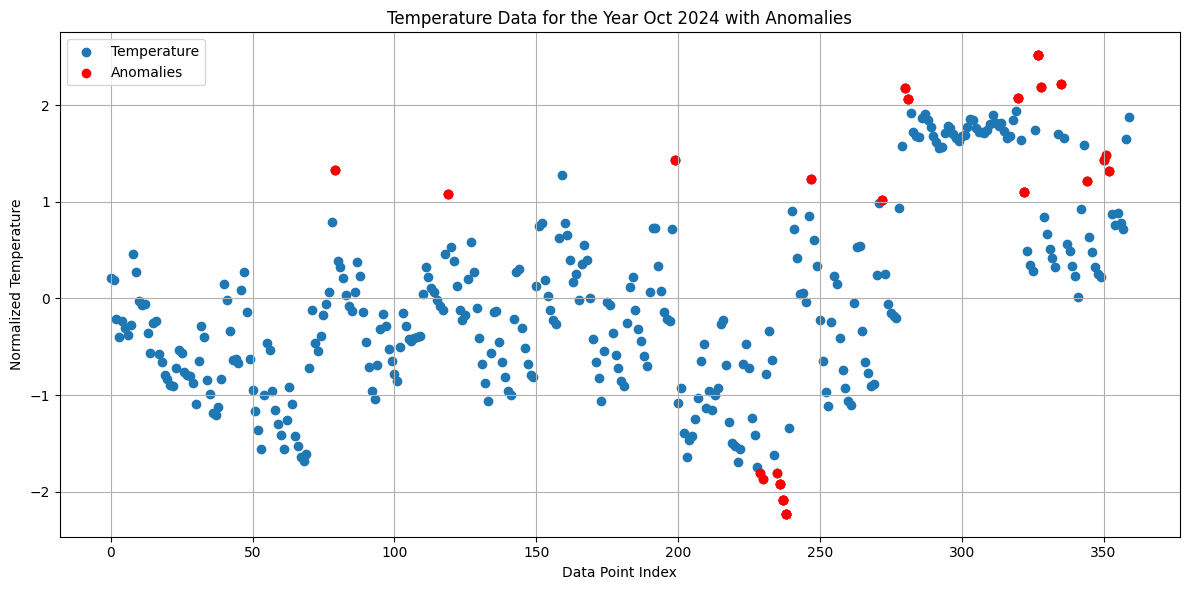
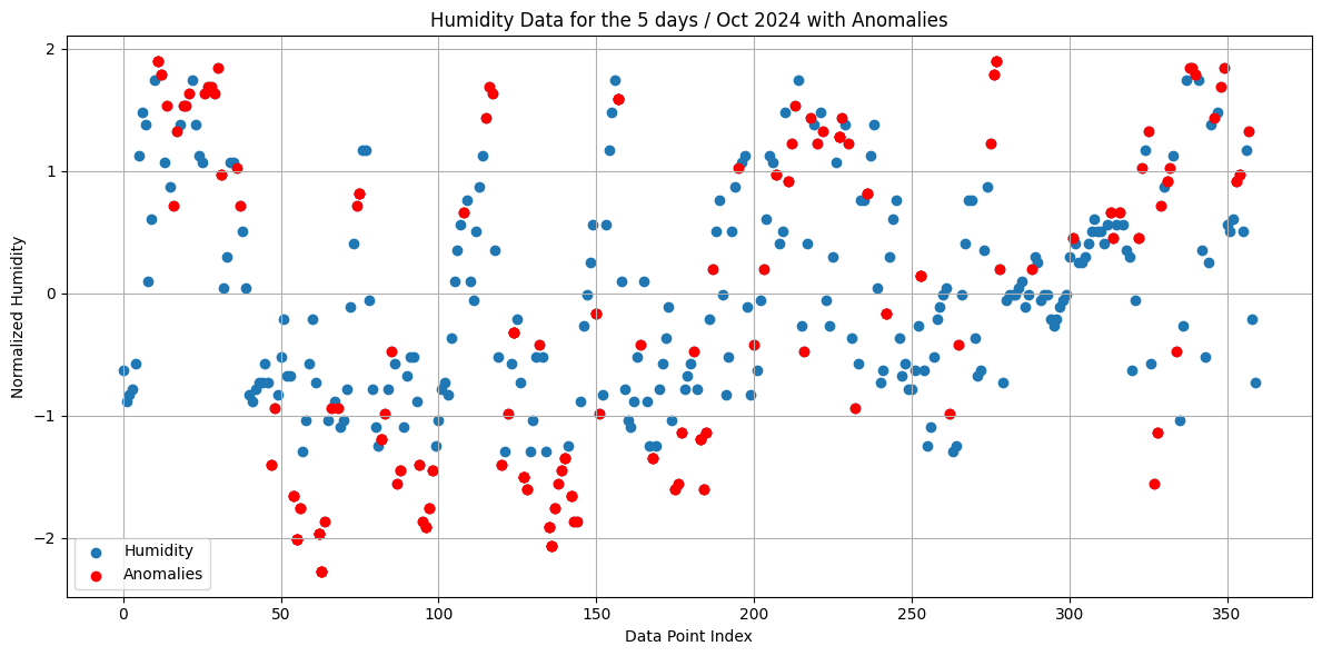
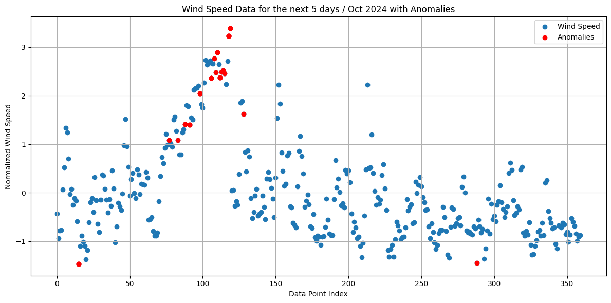
The red data points in Figures 3 to 5 represent anomalies, indicating unusual temperature variations or extreme weather conditions in Oct 2024 for the next 5 days, for the Temperature, Wind Speed and Humidity features.
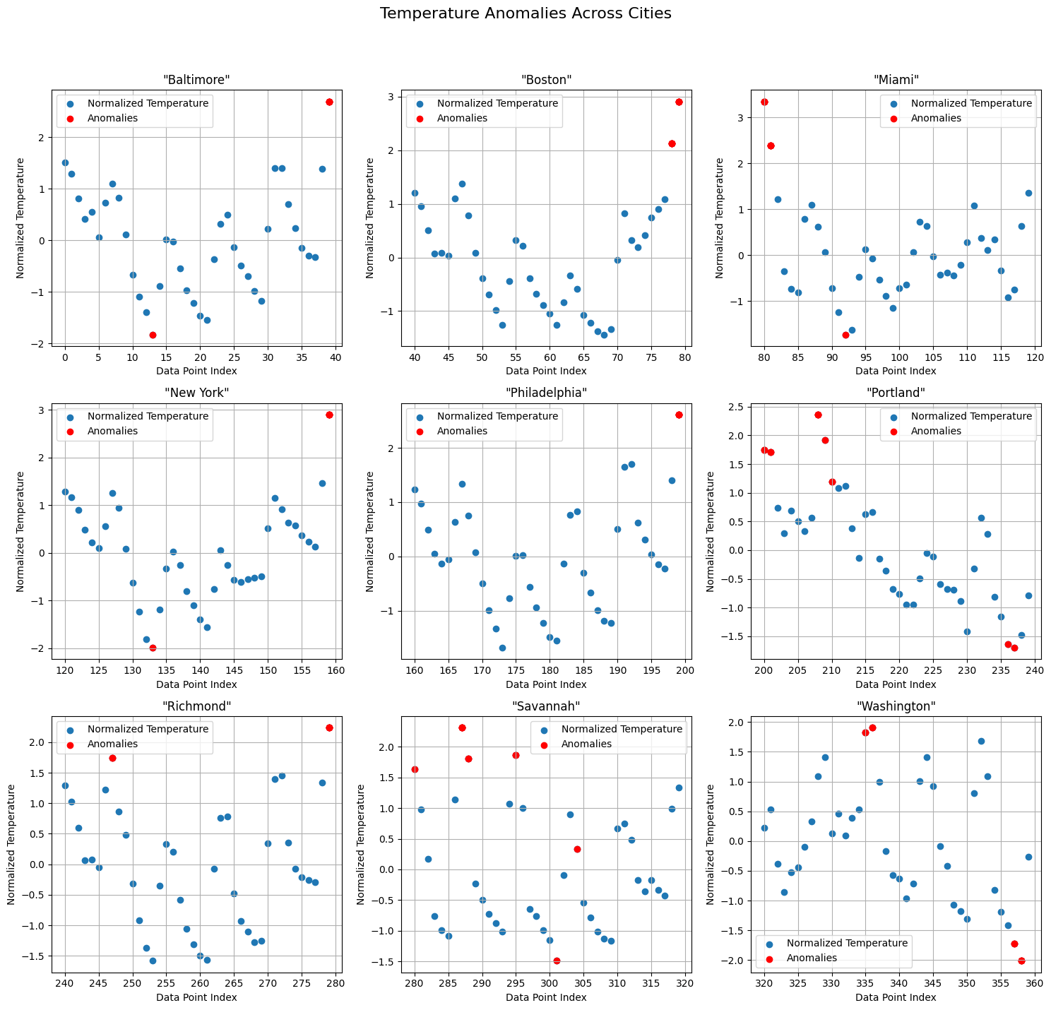
To show the plots for each city in a grid layout, Here’s how you can visualize it:
plaintextimport pandas as pd
import numpy as np
from sklearn.preprocessing import StandardScaler
from sklearn.neighbors import NearestNeighbors
import matplotlib.pyplot as plt
# Ensure the DataFrame is sorted by city and timestamp for easier plotting
df = df.sort_values(by=['city', 'forecast_time']).reset_index(drop=True)
# Set the parameters
k = 5
anomaly_threshold = 2.0 # Adjust as needed
# Get unique cities and determine grid size for plotting
cities = df['city'].unique()
n_cities = len(cities)
grid_cols = 3 # Number of columns in the grid
grid_rows = (n_cities + grid_cols - 1) // grid_cols # Calculate rows based on city count and columns
# Create a figure with a grid of subplots
fig, axes = plt.subplots(grid_rows, grid_cols, figsize=(15, 5 * grid_rows)) fig.suptitle('Temperature Anomalies Across Cities', fontsize=16)
axes = axes.flatten() # Flatten to handle axes indexing easily
# Loop through each city and plot on a grid
for i, city in enumerate(cities):
 # Filter data for the current city
 city_data = df[df['city'] == city].copy()
 # Normalize humidity values
 scaler = StandardScaler()
 city_data['temp_normalized'] = scaler.fit_transform(city_data[['temp_in_c']])
 # Train KNN model
 knn = NearestNeighbors(n_neighbors=k)
 knn.fit(city_data[['temp_normalized']])
 # Detect anomalies
 distances, _ = knn.kneighbors(city_data[['temp_normalized']])
 z_scores = ((distances - distances.mean()) / distances.std())

 # Identify anomalies for Humidity
 anomalies_humidity = city_data[z_scores > anomaly_threshold]
 # Plot the humidity data with anomalies highlighted
 ax = axes[i]
 ax.scatter(city_data.index, city_data['temp_normalized'], label='Normalized Temperatur e')
 ax.scatter(anomalies_humidity.index, anomalies_humidity['temp_normalized'], c='red', l abel='Anomalies')
 ax.set_title(f'{city}')
 ax.set_xlabel('Data Point Index')
 ax.set_ylabel('Normalized Temperature')
 ax.legend()
 ax.grid(True)
# Remove any empty subplots if n_cities is less than grid_rows * grid_cols for j in range(i + 1, len(axes)):
 fig.delaxes(axes[j])
plt.tight_layout(rect=[0, 0.03, 1, 0.95]) # Adjust layout to fit the title plt.show()In summary, we have applied unsupervised learning methods and statistical analysis to detect anomalies in temporal weather data. Through a variety of machine learning models we have succeeded in detecting anomalies in weather data.
Wrapping It Up
In conclusion, this approach demonstrates a robust solution for real-time data integration and analytics by using MongoDB, Estuary, and Databricks on Azure. By combining these technologies, you can efficiently capture and store dynamic weather data from the OpenWeather API, establish real-time data streaming with MongoDB change streams, and seamlessly transfer this data into Databricks for advanced analytics and visualization. Alternative methods, such as using the Apache Spark Connector for MongoDB, enable direct connectivity but require Spark coding and maintenance, which can add complexity, especially with continuous data synchronization.
In contrast, Estuary offers a streamlined, automated alternative that minimizes manual configuration and setup. With Estuary, real-time data pipelines maintain continuous data synchronization between MongoDB and Databricks, ensuring data accessibility and reliability. This architecture supports proactive decision-making, scalable growth, and operational efficiency, creating a strong foundation for data-driven insights and enabling quick detection of trends, patterns, and anomalies in real-time data.
Sign up for an Estuary account to start automating your data workflows and experience seamless data integration between varied sources and destinations apart from MongoDB to Databricks.
FAQs
How does Estuary ensure data consistency and reliability when integrating MongoDB with Databricks for real-time analytics?
Estuary employs several strategies to ensure data consistency and reliability during the integration of MongoDB with Databricks for real-time analytics:
- Change Data Capture (CDC): Estuary utilizes CDC to track changes in MongoDB, ensuring that only the latest data is ingested into Databricks. This minimizes the risk of data duplication and ensures that analytics are based on the most current information.
- Schema Evolution Support: Estuary supports schema evolution to account for schema changes, ensuring that MongoDB's data structure remains consistent and up-to-date without manual intervention.
- Transactional Guarantees: Utilizing exactly-once delivery semantics, Estuary ensures that each data record is processed only once, eliminating the risk of duplicates or data loss during transmission.
What advantages does Estuary offer over traditional ETL methods for real-time analytics with MongoDB and Databricks?
Estuary provides several advantages over traditional ETL methods, particularly for real-time analytics involving MongoDB and Databricks:
- Real-Time Data Ingestion: Estuary supports continuous data ingestion, allowing for real-time streaming of data into MongoDB. This is particularly beneficial for applications that require up-to-date information, such as dashboards and alerting systems.
- Low Code/No Code Approach: Estuary's low code/no code capabilities allow data engineers and analysts to set up pipelines quickly without extensive coding knowledge, speeding up the deployment of data integration solutions.
- Change Data Capture (CDC): Estuary supports change data capture, allowing for the efficient tracking of changes in data sources. This ensures that only the modified data is ingested, optimizing performance and resource utilization.
- Integration with Modern Data Stack: Estuary seamlessly integrates with modern tools and platforms, allowing for a streamlined workflow between MongoDB, Databricks, and other data services, enabling users to leverage advanced analytics and machine learning capabilities.
- Cost Efficiency: By minimizing the complexity of ETL processes and reducing the need for extensive infrastructure, Estuary can help lower operational costs associated with data ingestion and transformation.

About the author
Ruhee has a background in Computer Science and Economics and has worked as a Data Engineer for SaaS providing tech startups, where she has automated ETL processes using cutting-edge technologies and migrated data infrastructures to the cloud with AWS/Azure services. She is currently pursuing a Master’s in Business Analytics with a focus on Operations and AI at Worcester Polytechnic Institute.

