PostgreSQL is a powerful open-source database that supports materialized views. Traditional materialized views are database objects that contain the results of a query — usually, a focused subset of a large dataset. They’re powerful optimization tools. 

But what about materialized views of a real-time data feed? When you run a query at a set interval, you lose the real-time nature of your data. On its own, Postgres doesn’t support materialized views that update continuously. 

But that doesn’t mean it’s impossible to create one.

In this article, we’ll discuss an example workflow that uses Estuary Flow to create a real-time materialized view in Postgres, specifically focusing on Postgres CDC.

We’ll compare the dramatic difference in performance between queries on the raw data and the materialized view, and note the impact on our database’s CPU usage.

The raw and transformed datasets we use here are both publicly available from Estuary. At the end of this article, you’ll find steps to materialize them to your own database so you can test them however you’d like. 

Click here to skip straight to the DIY section. 

Note: As you read this article, you’ll encounter a couple of concepts unique to Estuary Flow. You might find it helpful to read this blog post for a quick primer. Relevant product documentation is also linked throughout.

The data: recent changes feed from Wikipedia

The Wikimedia Foundation offers a data stream of recent changes to its wikis, including Wikipedia, through its API. 

The Wikipedia recent changes stream is large: it captures every change to the platform — about 30 per second —  and includes various properties. Written to a Postgres table, it quickly grows to an unqueryable size. 

Let’s suppose we’re only interested in one aspect of this data: which Wikipedia editors are the most prolific. We only need to know how many changes each user makes on a given day, but we still want that information in real time. 

First attempt: Materialize the raw data feed 

Before we try to create a materialized view, our plan might simply be to ingest the entire real-time data feed into Postgres and query it as needed.

The methods to write a real-time data feed to Postgres vary widely, and can be tricky. But we kept it simple while creating this demo: we used Estuary Flow to capture the data feed.

We used a data connector to integrate with the real-time data feed from the Wikipedia API via an http endpoint. This created a data collection called estuary/public/wikipedia/recentchange (which is available publicly in Flow). 

Now, let’s imagine we try directly materializing that collection into a Postgres database. 

This yields a table in Postgres that contains all recent changes to Wikipedia, which quickly balloons in size. Below, we see the size of the data after just a few days. 

Repeatedly running a query against this table isn’t exactly the best use of compute resources. We may not have anticipated this problem when we first got ahold of the raw data; regardless, it’s now evident that we need to find a smarter way to isolate the data of interest.

So, we’ll use Flow to create a real-time materialized view: a pre-computed, continuously-updating fact table. 

Setup: Capture the data into Flow (if necessary)

As mentioned earlier, the raw Wikipedia data stream we’re using for this example comes from an HTTP endpoint, and it’s already available as a collection in Flow. 

However, there’s another common use case we should quickly address: one in which the raw data is already in your Postgres database, ingested through some other method. 

In that case, we’d need to capture the table from Postgres to create that collection. 

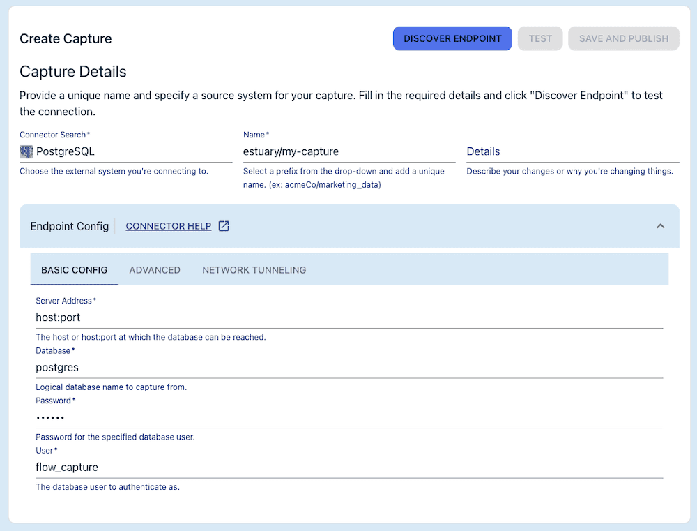
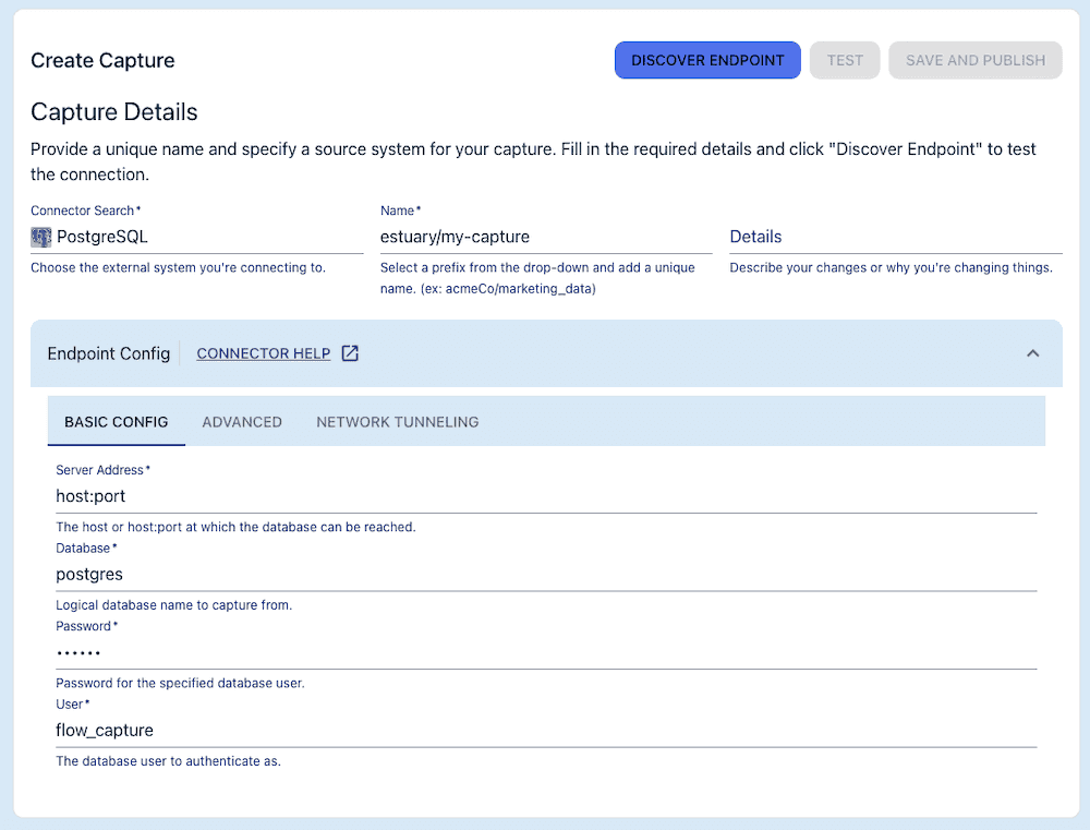
We’d do so in the Flow web app using the Postgres Change Data Capture connector. 

Step 1: Add a derivation to transform the data

Next, we will set up a Flow derivation. It’ll take our massive dataset and transform it into a small, efficient fact table that shows the number of updates each Wikipedia user makes on a given day. 

In other words, we’re replacing the need to run repeated SQL queries on our raw data table with a more efficient, pre-computed function.

Derivation creation is supported in local development environments using the flowctl command line tool. Using a TypeScript function and a new JSON schema for our data, we’ll derive a small fact table that contains only the user_id, the count of each user’s edits, and a last_updated date.

See the end of the article for steps to view the source files in your local environment and see how the derivation works under the hood.  

Step 2: Create the real-time materialized view

We’ve transformed the huge dataset into the smaller subset we’re interested in. Now, we simply go back to the Flow web app and materialize our new collection back into Postgres. 

Step 3: Compare performance

In our Postgres client application, it’s immediately clear that our materialized view is much smaller than our original dataset.

We can run a simple query and compare its execution statistics between the raw data…

…and the transformed data.

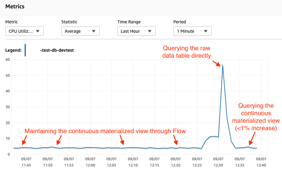
Perhaps most importantly, even if we’re running the full, end-to-end real-time materialized view (capturing the raw data from the database, transforming it, and then materializing back to the same database), we see minimal database CPU usage. The only time usage spikes is when we directly query the raw data.

Want to try it yourself?

Both the raw and transformed datasets are available for you to work with via the Estuary Flow web app. You can quickly materialize both datasets to your own Postgres database and compare performance. 

Requirements

• An Estuary Flow account. To start for free, head to the web app and fill in the registration form.
• Some familiarity with database administration. 

Materialize your own tables

1. Create a Postgres database in the hosting environment of your choice, or choose an existing database. Amazon RDS, Amazon Aurora, Google Cloud SQL, Azure Database for PostgreSQL, and self-hosted databases are supported.
2. Make note of the following properties. See the Flow docs for help finding them.
   1. A username and password for the instance.
   2. Your database host and port.
   3. The database name (if in doubt, use the default, “postgres”). 
3. Create a new materialization with Flow. 
   1. In the Flow web application, go to the Materializations page and click New Materialization. 
   2. For Connector, choose PostgreSQL. Add a unique name for the materialization, for example, yourOrg/yourname-materialized-views-demo. 
   3. Fill out the Basic Config with the properties you noted in step 2. 
   4. In the Collection Selector, search for and add the collection estuary/public/wikipedia/recentchange and name the corresponding Table wikipedia_raw. 
   5. Search for and add a second collection: estuary/public/wikipedia/user-fact-table. Name the corresponding Tablewikipedia_data_by_user.
4. Click Next to test the connection to the database and generate a configuration. 
5. Click Save and Publish.

In your Postgres client, both tables will become available for you to work with. 

Bonus: Explore the derivation

If you’re curious how the data was transformed, you can take a look at the derivation source files in your local environment. 

As you complete these steps, reference the guide to create a derivation. Though the derivation has already been created here, this guide will provide helpful context.

1. Install flowctl.
2. In the Flow web app, on the Admin Page, on the CLI-API tab, copy the access token. 
3. Authorize Flow locally: 
4. You’re now connected to Flow from your local environment. Start by creating a new Flow draft in which to work.
5. The new draft is empty. Add the derived collection to the draft:
6. Pull the files down for local work. They’ll be written to your working directory:
7. Generate a diagram of the files.

It will look like:

plaintext
.
├── estuary
│   └── public
│       └── wikipedia
│           ├── flow.yaml
│           └── user-fact-table.ts
├── flow.yaml
├── flow_generated
│   ├── flow
│   │   ├── main.ts
│   │   ├── routes.ts
│   │   └── server.ts
│   ├── tsconfig-files.json
│   └── types
│       └── estuary
│           └── public
│               └── wikipedia
│                   └── user-fact-table.d.ts
├── package.json
└── tsconfig.json

8. In the estuary/public/wikipedia subdirectory, open flow.yaml and user-fact-table.ts. 

The YAML file defines the Flow collection, and includes its schema with reduction annotations. These annotations merge the data based on user ID and the date they were last updated. 

The TypeScript file contains the transformation function, which counts the number of changes associated with each user on a given date. It also converts the timestamp in the source data to a familiar date format. 

What will you do with real-time materialized views?

If you use databases often, you’ve likely worked both with large, continuously-updating datasets, as well as query-based materialized views. 

Real-time materialized views give you the best of both worlds: real-time data with pre-computed transformations applied for efficiency. Using the method described in this post, they’re quite simple to set up — the hardest part is writing the transformation function. 

With your new Flow account, you’re free to move beyond the Wikipedia feed and experiment with your own data. 

Want to collaborate and get support as you take on more complex workflows? Join the Estuary Slack community.

plaintext
tree

plaintext
flowctl draft develop

plaintext
flowctl catalog draft --name estuary/public/wikipedia/user-fact-table

plaintext
flowctl draft create

plaintext
flowctl auth token –token your-token-here