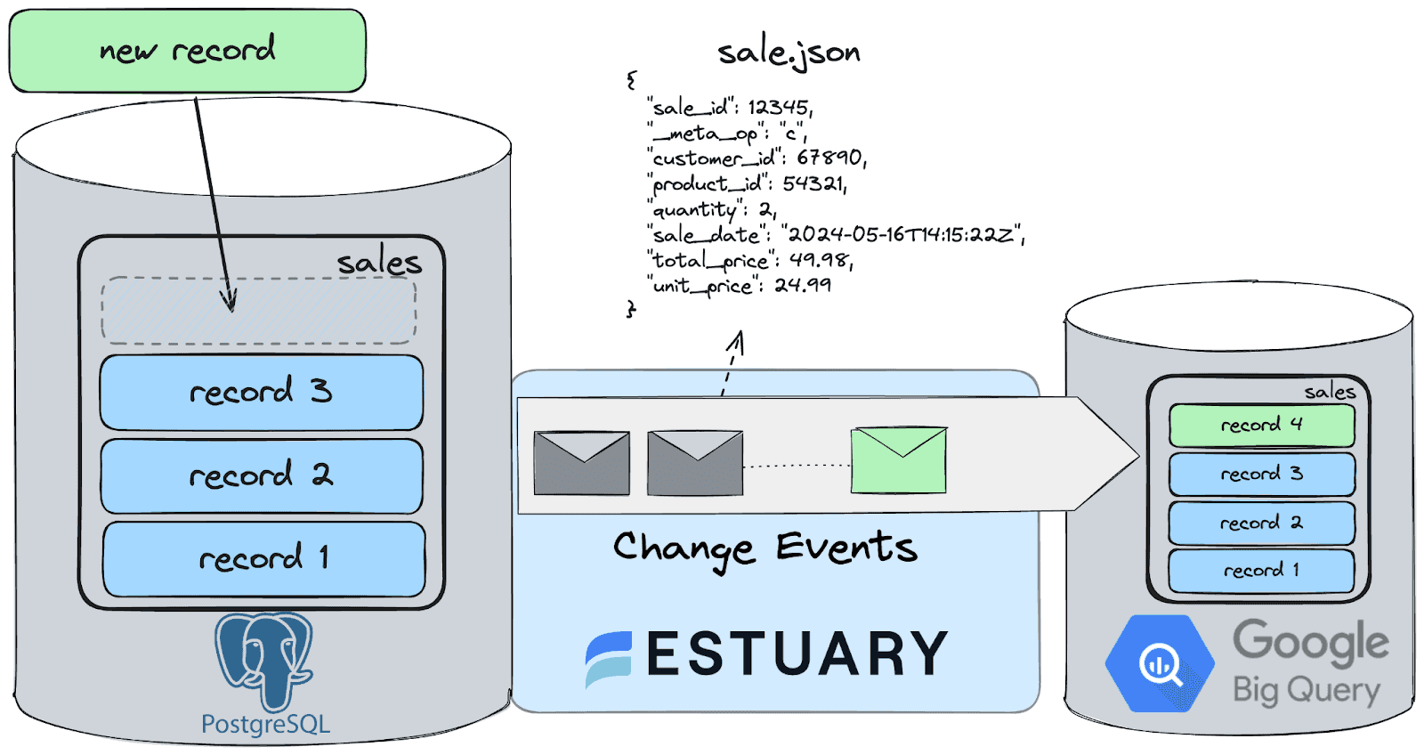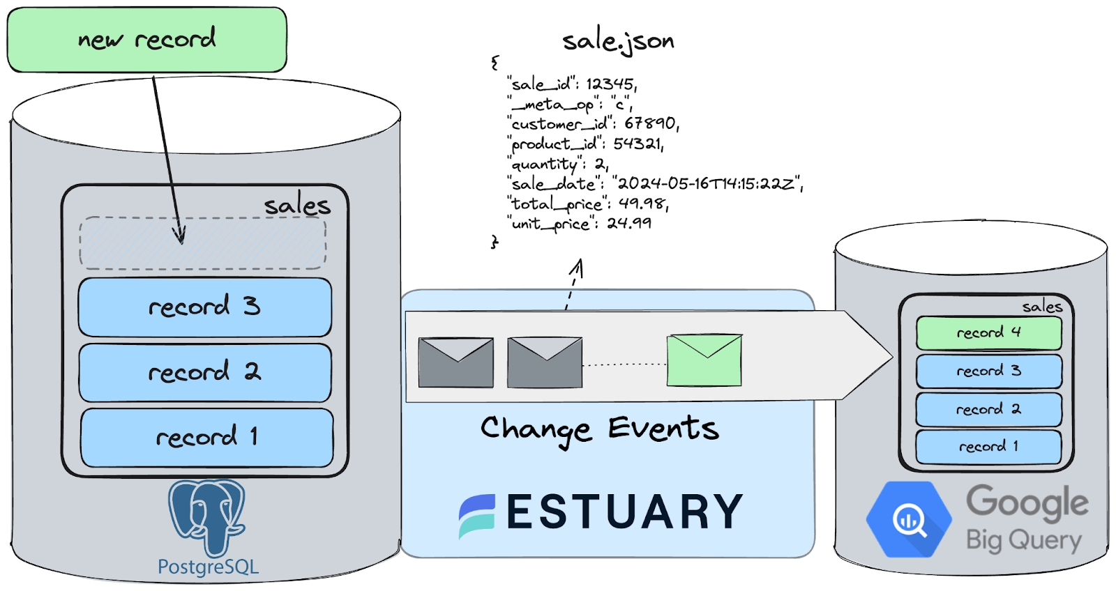
The purpose of this article is to build a realistic ELT pipeline using Estuary with dbt. I’m going to show you how to spin up a CDC connector that captures change events from a PostgreSQL database and loads them into BigQuery, where you’ll learn how to implement incremental models with dbt, to efficiently transform even the largest datasets.
You’ll utilize two features of Estuary that are critical for efficient and lean incremental analytical models in a data warehouse:
- flow_published_at Timestamp: By leveraging this timestamp, data practitioners can easily implement the incremental update process in dbt. Incremental models can efficiently process only new or updated data since the last run, improving performance and reducing processing time.
- _meta/op = ‘d’: Handling deletions effectively is crucial in maintaining accurate datasets. By filtering on the operation type fields provided by Estuary, dbt can identify and process deleted records, ensuring the transformed datasets accurately reflect the source data.
Let’s see how it works in practice!
Tools of the trade
Estuary is a real-time data integration platform designed for CDC and streaming. It excels at capturing data from various sources, transforming it on the fly, and delivering it to diverse destinations. With its event-driven architecture, Estuary ensures data is processed and delivered exactly once, with minimal latency, making it an ideal solution for modern data environments.
Some key features of Estuary are:
- Fully Integrated Pipelines: Estuary simplifies data integration by enabling you to create, test, and adapt pipelines that gather, modify, and consolidate data from multiple sources.
- Powerful Transformations: Estuary processes data using stable micro-transactions, guaranteeing committed outcomes remain unaltered despite crashes or machine failures.
- Connectors Galore: With pre-built connectors for popular data sources and sinks, such as databases and message queues, Estuary reduces the need for custom connectors. This speeds up data pipeline deployment and ensures consistency across systems.
dbt is a transformation framework that focuses on analytics engineering. It allows data practitioners to transform raw data into clean, analyzed datasets ready for business intelligence tools. dbt leverages SQL for data transformations, integrates seamlessly with various data warehouses, and promotes a modular, testable, and version-controlled approach to data transformation.
Some of the key features of dbt include:
- Version Control: dbt integrates well with version control systems like Git, enabling collaborative development, versioning, and change tracking.
- Data Testing: dbt provides a framework for writing tests to validate data quality and integrity. You can define tests for schema, uniqueness, null values, and more.
- Community and Ecosystem: dbt has a strong community and a growing ecosystem of tools, plugins, and resources that support various data warehousing platforms like Snowflake, BigQuery, Redshift, and more.
ELT (Extract, Load, Transform) is a data integration process where data is first extracted from source systems, then loaded into a data warehouse, and finally transformed into the desired format. This approach contrasts with ETL (Extract, Transform, Load) by deferring transformations until after the data has been centralized in the data warehouse, offering greater flexibility and scalability.
While Estuary does both ETL and ELT, this article focuses on enabling the latter, and letting dbt handle the transformations in the data warehouse.
Prerequisites
- Docker: For convenience, we are providing a docker compose definition which will allow you to spin up a database and a fake data generator service in about 5 seconds!
- ngrok: Estuary is a fully managed service. Because the database used in this tutorial will be running on your machine, you’ll need something to expose it to the internet. ngrok is a lightweight tool that does just that.
Step 1. Clone example repository and start up PostgreSQL
Head over to GitHub and clone the Estuary examples repository. Change directories into the one called postgres-cdc-bigquery-dbt. This folder contains the source PostgreSQL database container definition, the data generator script and the dbt project for the transformations in BigQuery.
First, spin up the containers.
plaintextexport NGROK_AUTHTOKEN=<your ngrok token>
docker compose up
After a few seconds, Docker will create three long-running services; one for the database, one for the Python script which continuously loads data into a table and third, ngrok, which exposes the database to the internet, so Estuary will be able to connect to it.
The init.sql script takes care of all the prerequisites needed to enable CDC, and it also creates the sales table which this data flow will replicate into BigQuery.
Step 2: Verify Data Insertion
Take a look at the logs of the data generator container to verify that records are being inserted into the table.
plaintextdocker logs datagen
Inserted new sale: (83, 57, datetime.datetime(2024, 4, 23, 2, 19, 37, 126905), 1, 69.83, 69.83)
Inserted new sale: (23, 348, datetime.datetime(2024, 4, 10, 3, 48, 29, 39255), 6, 99.51, 597.06)
Inserted new sale: (100, 495, datetime.datetime(2024, 2, 2, 8, 28, 5, 996012), 1, 73.25, 73.25)
Inserted new sale: (84, 724, datetime.datetime(2024, 4, 24, 0, 26, 41, 411600), 3, 19.35, 58.05)
Inserted new sale: (61, 448, datetime.datetime(2024, 3, 18, 2, 17, 14, 96383), 10, 59.09, 590.9)
Deleted sale ID 1063
Updated sale ID 654 with new data: (50, 796, datetime.datetime(2024, 1, 14, 2, 2, 57, 161933), 10, 20.3, 203.0)
Deleted sale ID 406
Step 3: Expose Database with ngrok
Looks good! The last step is to grab the public URL of the database.
plaintextcurl -s http://localhost:4040/api/tunnels | jq -r '.tunnels[0].public_url'
tcp://5.tcp.eu.ngrok.io:19236
Great, it’s time to start capturing change events.
Step 4: Configure PostgreSQL Capture in Estuary
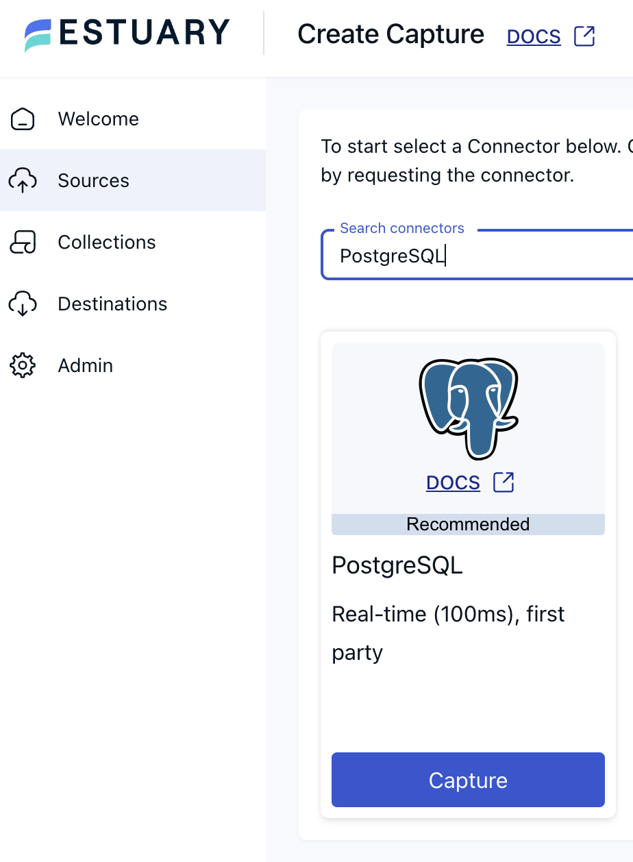
Head over to the Estuary dashboard and create a new PostgreSQL capture.
During the endpoint configuration, use the URL from the previous step and for the user/password combination, the PostgreSQL container is configured as postgres/postgres. After pressing next, in the following section, you can configure how the incoming data should be represented in Flow.
Step 5: Deploy Connector and Verify Data Capture
For the sake of this tutorial, feel free to leave everything at its default setting and press Next again, then Save and Publish to deploy the connector and kick off a backfill.
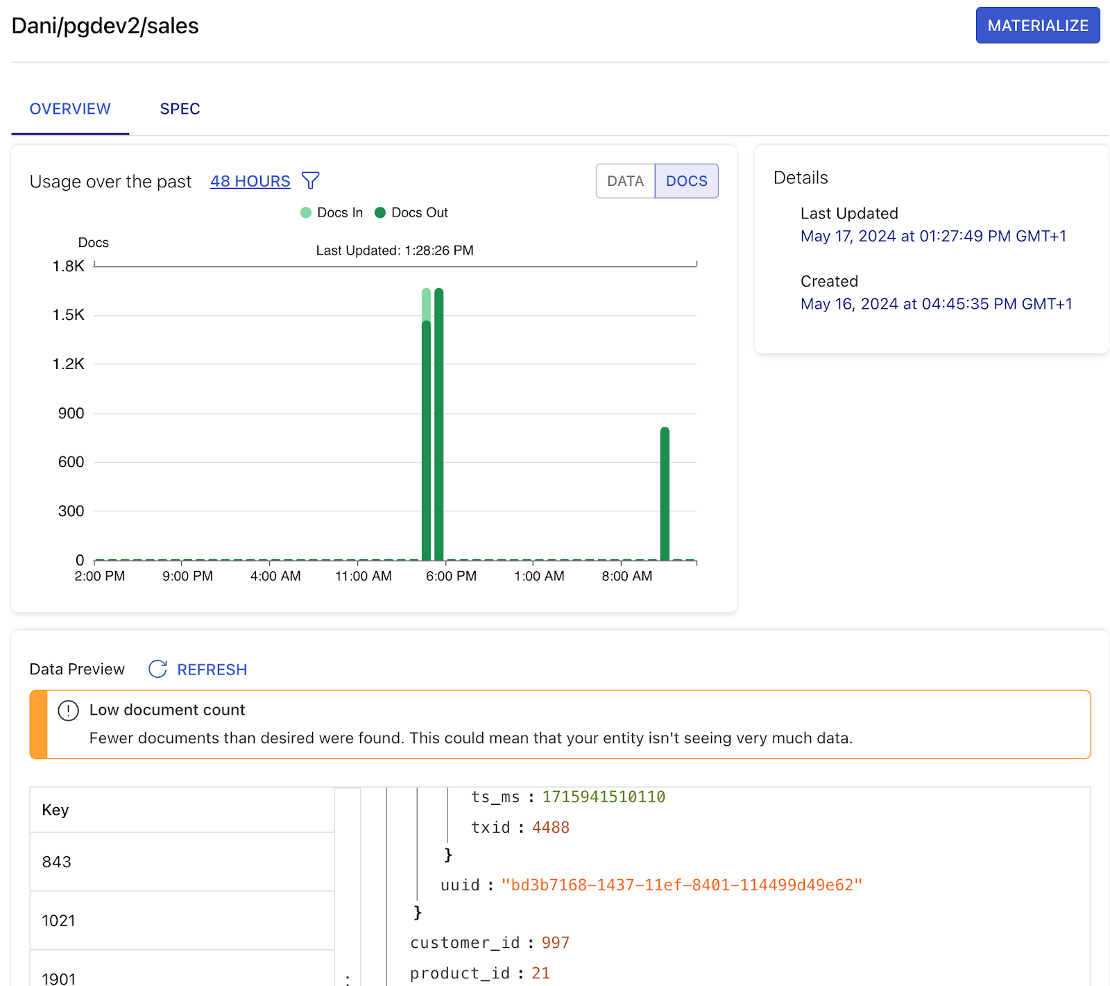
After the connector is successfully deployed, head over to the Collections page and take a look at the new sales collection.
This is where all change events captured by the connector coming from the source’s sales table are going to land as documents.
The documents of your flows are stored in collections: real-time data lakes of JSON documents in cloud storage. Documents being backed by an object storage mean that once you start capturing data, you won’t have to worry about it not being available to replay – object stores such as S3 can be configured to cheaply store data forever. See docs page for more information.
Step 6: Configure BigQuery Materialization
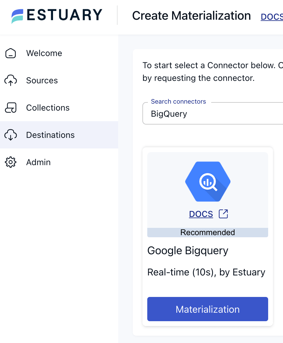
The goal of this tutorial is to move data into BigQuery, so let’s continue with that. As this is an ELT dataflow, there’s no need to do any transformations before the data lands in BigQuery. Head over to the Destinations page to create a new materialization and search for the BigQuery connector.
To use this connector, you'll need:
- A new Google Cloud Storage bucket in the same region as the BigQuery destination dataset.
- A Google Cloud service account with a key file generated and the following roles:
- roles/bigquery.dataEditor on the destination dataset
- roles/bigquery.jobUser on the project with which the BigQuery destination dataset is associated
- roles/storage.objectAdmin on the GCS bucket created above
To configure your service account, complete the steps available in the connector documentation. After all the details are in place, take a look at the Update Delay parameter.
The Update Delay parameter in Estuary materializations offers a flexible approach to data ingestion scheduling. It represents the amount of time the system will wait before it begins materializing the latest data.
For example, if an update delay is set to 2 hours, the materialization task will pause for 2 hours before processing the latest available data. This delay ensures that data is not pulled in immediately after it becomes available. For this tutorial, let’s set it to 0s, as in zero seconds, in order to demonstrate the flow in real-time.
After the connection details are in place, the next step is to link the capture you just created to Estuary and ensure it's able to see collections you are loading data into from Postgres. Press Next, then Save and Publish in the top right corner to provision the materialization connector.
Head over to the BigQuery console to verify that data is being loaded.
Step 7: Configure dbt for Incremental Models
So far, you have set up the extraction and loading steps of the data flow. While in a traditional ETL pipeline you would do transformations before data lands in the target system, here the goal is to replicate the incoming data in a form as close to the source as possible and execute the transformations on the destination side.
Let’s take a look at how the change events being streaming from Estuary enable efficient incremental models with dbt. In the project folder, change into the sales_dbt_project directory. This folder contains the dbt project.
If you haven’t already you can configure access to BigQuery from dbt by running the following:
plaintextdbt initAfter you’re set, take a look at the lineage of the models defined.
It’s a fairly small DAG; there are 2 downstream models after the source table, which is the one Estuary is streaming data into.
stg_sales simply selects the records needed for the incremental model and if you wanted to do any preliminary data cleaning it would go here as well.
sales on the other hand, looks like a bit more complex:
Step 8: Implement and Run Incremental Models with dbt
plaintext{{
    config(
        materialized='incremental'
    )
}}
with source as (
    select * from {{ ref('stg_sales') }}
)
select
  sale_id,
  _meta_op,
  customer_id,
  flow_published_at,
  product_id,
  quantity,
  sale_date,
  total_price,
  unit_price,
  flow_document
from source
where _meta_op != 'd'
{% if is_incremental() %}
  -- this filter will only be applied on an incremental run
  -- (uses >= to include records whose timestamp occurred since the last run of this model)
  and flow_published_at >= (select coalesce(max(flow_published_at), '1900-01-01') from {{ this }})
{% endif %}
You can see here that the model is using two neat features of Estuary. It’s filtering out the deleted documents using the _meta_op field and it defines an incremental filter as well, based on the flow_published_at field.
The flow_published_at field is a crucial component derived from the Estuary runtime. It represents the timestamp when a document (or JSON object) is captured and published to the collection. This field is available in every collection and serves as a proxy for the time when the document was last changed.
For example, in this flow, flow_published_at can be used as an updated_at value. This allows for efficient incremental transformations in BigQuery by processing only the data that has been captured or updated since the last run. By filtering records based on flow_published_at, you can ensure that only new or modified data is processed, significantly enhancing the performance and efficiency of incremental models.
Take it for a spin by executing the following command:
plaintextdbt run
12:51:50  Running with dbt=1.8.0
12:51:50  Registered adapter: bigquery=1.8.1
12:51:50  Found 2 models, 1 source, 469 macros
12:51:50
12:51:52  Concurrency: 1 threads (target='dev')
12:51:52
12:51:52  1 of 2 START sql view model dani_dev.stg_sales ................................. [RUN]
12:51:53  1 of 2 OK created sql view model dani_dev.stg_sales ............................ [CREATE VIEW (0 processed) in 1.31s]
12:51:53  2 of 2 START sql incremental model dani_dev.sales .............................. [RUN]
12:51:57  2 of 2 OK created sql incremental model dani_dev.sales ......................... [MERGE (560.0 rows, 1022.9 KiB processed) in 3.70s]
12:51:57
12:51:57  Finished running 1 view model, 1 incremental model in 0 hours 0 minutes and 6.51 seconds (6.51s).
12:51:57
12:51:57  Completed successfully
12:51:57
12:51:57  Done. PASS=2 WARN=0 ERROR=0 SKIP=0 TOTAL=2
You will be able to observe that for the first run, the incremental model will process all of the rows that exist in the source table. Try running the same command again to see how it behaves with new data! If everything works properly the incremental model should only process the records which arrived later in time compared to the first execution.
Conclusion
By combining Estuary and dbt, we leaned on the strengths of both platforms to create a robust and efficient CDC pipeline. This integration allowed us to automate data ingestion, streamline transformations, and maintain high data quality, ultimately enabling more informed and timely business decisions.
The flow_published_at field and the ability to handle deleted records with meta/op = ‘d’ proved to be useful features, optimizing our incremental model definitions and ensuring that our data was always up-to-date.
In summary, Estuary and dbt are a perfect match for modern ELT pipelines.
We hope this tutorial has provided you with the knowledge and tools to implement your own CDC pipeline and leverage the full potential of Estuary and dbt in your data transformation projects.
If you want to learn more, make sure you read through the Estuary documentation.
You’ll find instructions on how to use other connectors here. There are more tutorials here.
Also, don’t forget to join the Estuary Slack Community!

About the author
Dani is a data professional with a rich background in data engineering and real-time data platforms. At Estuary, Daniel focuses on promoting cutting-edge streaming solutions, helping to bridge the gap between technical innovation and developer adoption. With deep expertise in cloud-native and streaming technologies, Dani has successfully supported startups and enterprises in building robust data solutions.

