Building a Streaming Lakehouse with Estuary Flow and Apache Iceberg

Introduction

A streaming lakehouse is essentially the same as a regular data lakehouse, with the addition of a streaming ingestion layer. From a data consumer perspective, this doesn’t change many things, except that the data available will always be fresh.

On the technical side, there are a lot of challenges, as table formats (the governance layer over a data lake’s flat files) are not necessarily built for efficient streaming data ingestion. In a streaming environment, data is loaded row-by-row, but parquet files are written column-by-column.

In this tutorial, you will learn how to build a basic streaming lakehouse using Estuary Flow for the ingestion layer, Apache Iceberg as the table format, and PyIceberg as the query engine for the analytical transformations.

Components for Building a Streaming Data Lakehouse

Let’s take a look at the tools we’re going to use for the streaming lakehouse.

• Estuary Flow: Flow is the real-time data integration layer that will capture all changes from a PostgreSQL database using change data capture (CDC) and materialize them as Iceberg tables.
• Apache Iceberg: Apache Iceberg is a table format that enhances flat files in a data lake with capabilities such as transactions, version control, and other features.
• PyIceberg: PyIceberg is a Python-based client library to interact with Iceberg tables. We’ll be using it as a “compute engine” combined with the pandas library to query and transform data from the Iceberg tables.

Prerequisites

If you wish to follow along with the tutorial, all you’ll need are:

• An Estuary Flow account. You can register for free here.
• An AWS account to store the parquet files for the Iceberg tables.
• All code referenced in the article is available here.

And that’s it!

Step 1: Ingest Data into Estuary Flow

In this use case, a company wants to leverage real-time data integration to gain timely insights into user activity and transaction patterns. The dataset includes three interrelated tables: users, transactions, and transaction_metadata, representing user profiles, transactions, and metadata associated with each transaction.

The company wants to capture changes to this data in real time, enabling downstream applications to monitor and respond to critical events, such as new user registrations, high-value transactions, and flagged transaction metadata (such as suspicious activity).

Estuary Flow will capture inserts, updates, and deletes from these tables, ensuring the downstream data in the Iceberg tables is always up-to-date.

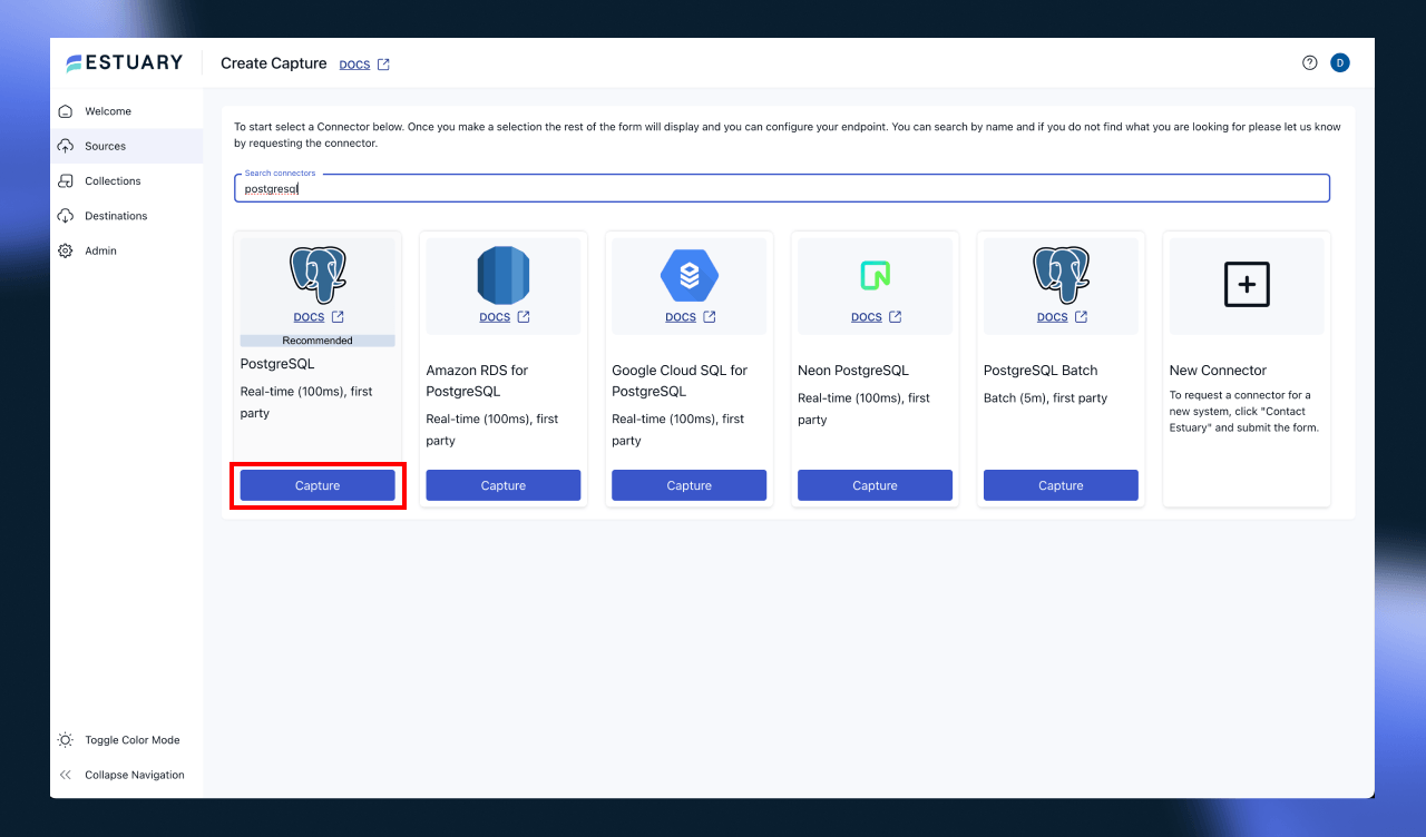
To start ingesting data, head to the Flow dashboard and create a new PostgreSQL capture.

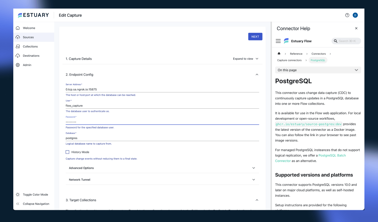
After clicking the “Capture” button, you must configure the connection details so Flow can access the database. If you’re using the example docker image, the database is pre-configured to allow change data capture.

Otherwise, head to the docs page to learn more about the connector requirements.

Feel free to leave all the configuration settings as the default ones, they will be sufficient for this tutorial.

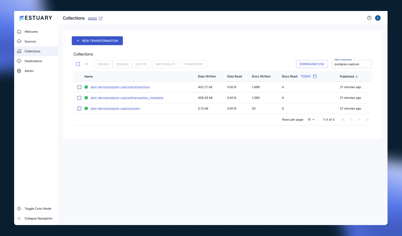
Once the connector is provisioned, after a few seconds, you’ll see data being ingested into Flow collections. Collections are the internal data structure of Flow. They are JSON files stored in an object storage, such as S3.

You can configure Flow to use your own object storage for extra governance if you want, although not necessary.

Step 2: Configure Apache Iceberg Materialization

Once the PostgreSQL connector is actively capturing data, the next step is to materialize the collections in Iceberg. To achieve this, we’ll need to set up the Iceberg Materialization connector.

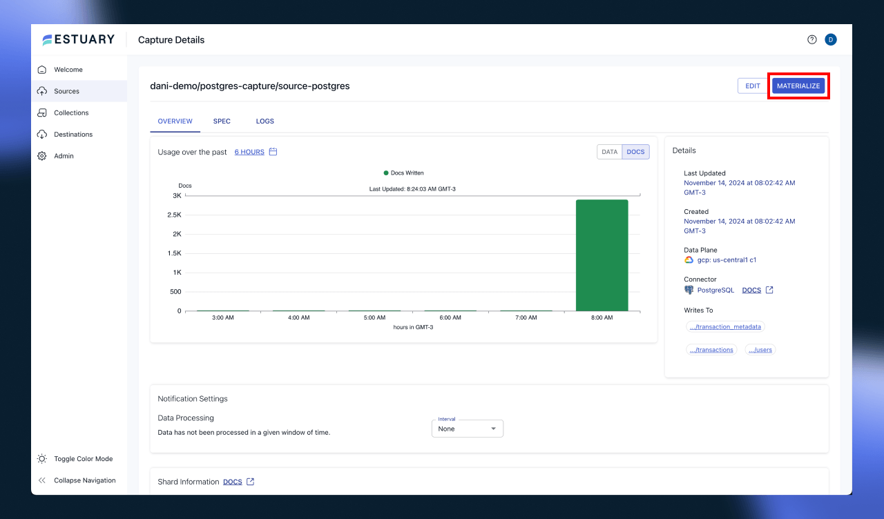
Head over to the capture connector’s page and press the “Materialize” button.

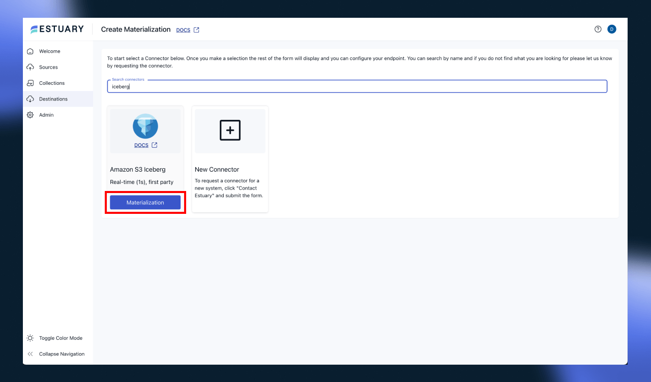
Look for the Amazon S3 Iceberg connector.

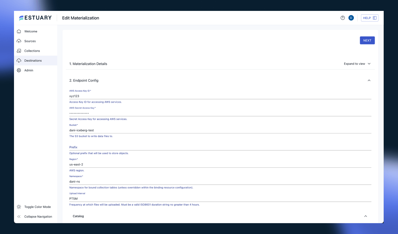
This will navigate to the connector configuration page, which is similar to the previous step. There, you’ll 

have to enter your AWS credentials and set some other parameters for the connector.

Make sure to note the value for the Upload Interval configuration setting. This setting defines how often Flow will kick off a materialization into Iceberg. It’s important to consider the tradeoff between data freshness and the “small file problem”. If you are not implementing compaction, you’ll notice a considerable performance degradation once you start running analytical queries that need to read many thousands or more small files.

For the tutorial, it’s totally fine to leave it as PT5M, which means Flow will materialize data every 5 minutes.

For the catalog, we’re going to choose Glue for this tutorial, but if you have a REST catalog ready to be used, feel free to choose that option!

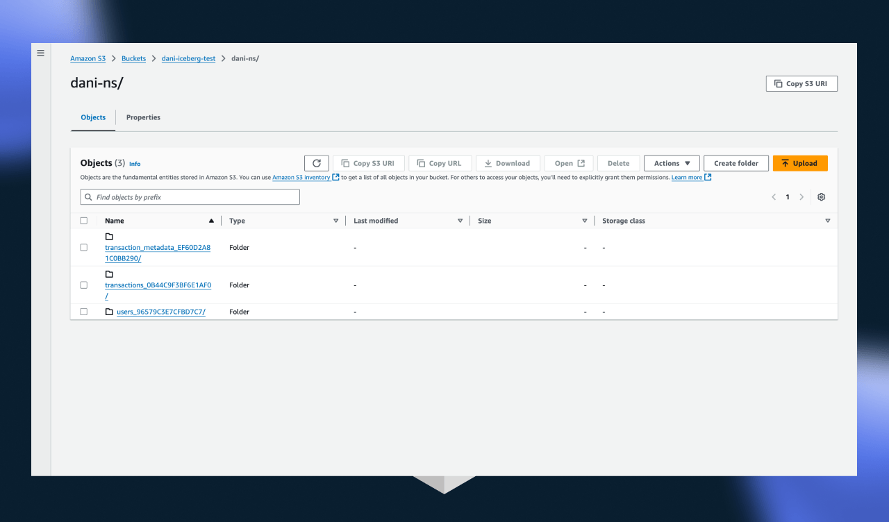
Once you’re done and the connector is created, you can sneak a peek of the results by navigating to the S3 bucket you’ve configured as the destination.

You should see 3 prefixes for the 3 tables the connector is materializing.

Great, it looks like data is being materialized from Flow into Iceberg tables! Let’s take a look at how we can start analyzing with PyIceberg and pandas.

Step 3: Query the Iceberg Table Using PyIceberg

Now for the fun part! Let’s take a look at how we are able to access data lakehouse we just created.

PyIceberg is a Python client for Apache Iceberg. It allows Python developers to interact with Iceberg tables, making it easier to work with the Iceberg format directly in Python-based data environments.

You can install it by running the following:

plaintext
pip install "pyiceberg[glue]"

Make sure to include the glue extension, as that’s the catalog we’re using for our lakehouse!

Let’s take a look at how we can query the tables using Python:

python
from pyiceberg.catalog.glue import GlueCatalog

table = catalog.load_table(f"{os.getenv('NAMESPACE')}.transactions")

df = table.scan().to_pandas()

print(df.describe())

print(df.head())

This script will load the data from the transactions table and morph it into a pandas data frame. If you run this snippet, the results should look something like this:

python
       transaction_id       amount      user_id
count     5274.000000  4323.000000  4323.000000
mean      1862.004930   749.226438    10.540365
std       1107.154199  1324.346755     5.764058
min          2.000000     0.010000     1.000000
25%        902.250000   240.485000     6.000000
50%       1760.500000   517.420000    10.000000
75%       2780.750000   783.500000    16.000000
max       3991.000000  9934.970000    20.000000

   transaction_id  ...                                      flow_document
0              55  ...  {"_meta":{"op":"d","source":{"loc":[29622752,2...
1             150  ...  {"_meta":{"op":"u","source":{"loc":[29697608,2...
2             154  ...  {"_meta":{"op":"u","source":{"loc":[29600688,2...
3             174  ...  {"_meta":{"op":"d","source":{"loc":[29669512,2...
4             181  ...  {"_meta":{"op":"d","source":{"loc":[29601200,2...

[5 rows x 7 columns]

Process finished with exit code 0

Great, although we have to keep in mind that these values are for the raw change data, which can be misleading. If we want to use the change records located in the flow_document for most analytics use cases, we’ll have to merge them into their latest state. Luckily, this can be done quickly with pandas!

python
# Function to extract operation type from the flow_document JSON field
def get_operation(flow_document):
    try:
        doc = json.loads(flow_document)
        return doc["_meta"]["op"]
    except (json.JSONDecodeError, KeyError):
        return None

# Add a column for the operation (insert, update, delete)
df['operation'] = df['flow_document'].apply(get_operation)

# Filter updates and deletes
updates_df = df[df['operation'] == 'u']
deletes_df = df[df['operation'] == 'd']

# Filter insertions (operations that aren't 'u' or 'd') - assuming these are additions
insertions_df = df[~df['operation'].isin(['u', 'd'])]

# Remove deleted transactions from the original DataFrame (i.e., filter out 'd' operations)
df_remaining = df[~df['operation'].isin(['d'])]

# Merge updated transactions into the remaining DataFrame
merged_df = pd.concat([df_remaining, updates_df]).drop_duplicates(subset=['transaction_id'], keep='last')

# Now, 'merged_df' contains the latest state of the transactions table
print(merged_df.describe())
print(merged_df.head())

Using the above snippet, we essentially reconstruct the table's original format. Now, we can start analyzing!

python
aggregated_df = df.groupby('user_id')['amount'].sum().reset_index()
aggregated_df.rename(columns={'amount': 'total_transaction_amount'}, inplace=True)
print(aggregated_df)

    user_id  total_transaction_amount
0       1.0                 168671.50
1       2.0                 170967.18
2       3.0                 165466.74
3       4.0                 181046.91
4       5.0                 176075.18

Awesome, this is exactly what we wanted. If you transform the other tables similarly, you can easily start joining the datasets together to compose more complex transformations.

Conclusion

In this article, we have walked through the steps to set up a basic streaming lakehouse architecture using Estuary Flow, Apache Iceberg, and PyIceberg.

By connecting Estuary Flow to your data source, enabling change data capture (CDC) for real-time ingestion, and storing the data in Iceberg tables, we’ve demonstrated how to create a powerful, scalable, and efficient architecture. PyIceberg then enables you to query and analyze this data with minimal setup, leveraging the full power of Iceberg’s data management capabilities.

The streaming lakehouse architecture offers significant advantages for real-time data analysis, including seamless data ingestion, easy schema evolution, and robust querying capabilities.

With this setup, you can ingest data continuously, perform real-time analytics, and gain valuable insights from streaming data in near real-time. Iceberg's support for large datasets and its time travel features provide a solid foundation for managing both batch and real-time workloads.

Next Steps

As you continue to build your streaming lakehouse, here are a few next steps to consider:

• Scaling the Lakehouse: As your data volume increases, you can scale the ingestion process and optimize Iceberg's storage to handle larger datasets with partitioning and clustering strategies.
• Incorporating More Data Sources: Expand the lakehouse by adding more data sources for ingestion, such as Kafka, cloud storage, or other databases. Estuary Flow supports integration with a variety of data sources to enable a truly unified pipeline.
• Exploring Advanced Iceberg Features: Dive deeper into Iceberg's advanced features, such as schema evolution, partition evolution, and ACID transactions, to further optimize your data lakehouse and ensure it supports the needs of your evolving workloads.

Additional Resources

• Estuary Flow Documentation: Learn more about how to set up and use Estuary Flow for real-time data ingestion and change data capture -> Estuary Flow Docs.
• Apache Iceberg Documentation: Dive into Iceberg's table format, partitioning strategies, and time travel capabilities Apache Iceberg Docs.
• PyIceberg Documentation: Get started with PyIceberg to query and analyze data stored in Iceberg tables PyIceberg Docs.
• Further Reading on Streaming Lakehouses: Explore more about the best practices around loading data into Iceberg.

By following the steps outlined and exploring the additional resources, you can build a robust, scalable streaming lakehouse that supports real-time data analytics and future-proofs your data architecture.

As always, don’t forget to join the Estuary Slack Community!