Introduction
Apache Parquet is an open-source columnar storage format designed for efficient data storage and retrieval. Developed as part of the Apache Hadoop ecosystem, Parquet has become a standard in data warehousing and big data analytics due to its high performance and efficiency.
It was initially created to support the needs of Hadoop frameworks like Apache Hive, Apache Drill, and Apache Impala, and has since been widely adopted in various data processing tools and platforms.
Data lakes, such as Apache Iceberg and Delta Lake, also rely heavily on Parquet as a common storage format. Although these data lakes have different architectures and functionalities, including features like transaction support, schema management, and data versioning, they both leverage Parquet's columnar storage to optimize data retrieval and analytics. This shared reliance on Parquet underscores its versatility and efficiency in managing large-scale data environments.
In this article, we’ll explore the history of Apache Parquet and take a look at the reasons why it became so popular.
History and Origins of Apache Parquet
Apache Parquet was born out of the need for a more efficient and performant columnar storage format for the Hadoop ecosystem. The project was initiated by engineers from Twitter and Cloudera, who recognized the limitations of existing storage formats and sought to create a solution that could better handle the demands of big data analytics.
Parquet was designed as an improvement on the Trevni columnar storage format created by Doug Cutting, the creator of Hadoop. The goal was to design a storage format that could provide high performance for read-heavy workloads typical in data analytics, while also being efficient in terms of storage space. The design was heavily influenced by Google’s Dremel paper, which described the columnar storage format used in Google BigQuery.
The Early Days
In March 2013, the first version of Apache Parquet was released. It quickly gained attention for its ability to significantly improve the performance of read-heavy analytical queries by reducing the amount of data that needed to be read from disk. Parquet achieved this through its columnar storage layout, which allowed for more effective compression and efficient scanning of relevant columns.
Parquet’s design made it an attractive choice for a variety of big data processing frameworks. Apache Hive and Apache Pig were among the first to integrate Parquet support, allowing users to leverage its performance benefits within their existing Hadoop workflows. Apache Drill, Apache Impala, and Apache Spark soon followed, further cementing Parquet’s position as a go-to storage format in the Big Data ecosystem.
Parquet's Role in Data Lake Architectures
The rise of data lakes brought new requirements for efficient and flexible storage formats. Apache Parquet’s attributes made it a natural fit for these environments. Data lakes like Apache Iceberg and Delta Lake adopted Parquet as their underlying storage format, leveraging its performance and compression benefits while adding features like ACID transactions and advanced schema management on top.
Let’s dive deeper into what features make Parquet so popular.
How Apache Parquet Works: Internals and Key Features
Apache Parquet's design and implementation draw significant inspiration from the striping and assembly algorithms outlined in the Dremel paper from Google. These algorithms are crucial for efficiently storing and retrieving data in a columnar format, optimizing performance and storage efficiency.
How Parquet Organizes Data into Columns: The Striping Algorithm
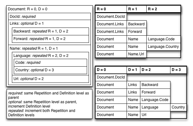
In Apache Parquet, the column striping algorithm is pivotal for organizing data into its columnar structure. This algorithm can be visualized as a depth-first traversal of a schema-defined tree structure, where each leaf node corresponds to a primitive-type column.
Let's illustrate this with an example based on the schema from the Dremel paper based on these notes by Julien Le Dem (Apache Parquet co-creator) :
plaintextmessage Document {
  required int64 DocId;
  optional group Links {
    repeated int64 Backward;
    repeated int64 Forward;
  }
  repeated group Name {
    repeated group Language {
      required string Code;
      optional string Country;
    }
    optional string Url;
  }
}
For this schema, Apache Parquet would generate columns as follows:
plaintextDocId
Links.Backward
Links.Forward
Name.Language.Code
Name.Language.Country
Name.Url
The striping algorithm involves:
- Serializing a record by traversing the tree from the root to the leaves.
- Writing values for each column at the maximum definition level (indicating the value is defined) and the current repetition level (starting from 0 at the root).
For instance, serializing a record might look like this:
plaintextDocId: 10, R:0, D:0
Links.Backward: NULL, R:0, D:1 (no value defined, so D < 2)
Links.Forward: 20, R:0, D:2
Name.Language.Code: 'en-us', R:0, D:2
Name.Language.Country: 'us', R:0, D:3
Name.Url: 'http://A', R:0, D:2
This approach efficiently encodes the data with minimal overhead, leveraging repetition and definition levels to manage nested and repeated structures effectively.
Record Assembly in Parquet: Reconstructing Data Efficiently
The record assembly process in Apache Parquet reverses the serialization process. It reconstructs records by traversing the tree structure based on the columns required.
This process allows efficient access to specific fields without needing to read unnecessary data, thereby optimizing query performance.
Repetition and Definition Levels
In Parquet, repetition and definition levels play crucial roles in managing nested and repeated data structures:
- Repetition Level (R): Indicates the depth of nesting for repeated fields. It increments when traversing repeated fields, allowing efficient reconstruction of repeated elements.
- Definition Level (D): Indicates whether a value is defined (present) or undefined (null). It increments when traversing optional fields, ensuring that only valid data is processed.
These levels are encoded efficiently using a compact representation, optimizing storage and processing efficiency.
Apache Parquet's adoption of concepts from the Dremel paper underscores its commitment to providing high-performance, scalable data storage solutions.
These foundational principles not only enhance Parquet's capabilities in data lakes and analytics platforms but also contribute to its widespread adoption as a preferred storage format in modern data architectures.
Row-Based vs. Columnar Storage: A Comparison
A file format acts as a set of rules that specify how information is structured and organized within a file. These rules determine how data is stored, the types of data allowed, and the methods used to interact with and modify the data. File formats vary depending on the specific data they handle and their intended purposes. For instance, text files such as TXT or DOCX are designed for textual content, while formats like JPEG or PNG are optimized for images.
When it comes to data formats, some of the most commonly used ones include CSV, JSON, and XML. Additionally, there are less familiar formats made for more specialized use cases, like Avro, Protocol Buffers, and Parquet.
What does the “columnar” part mean?
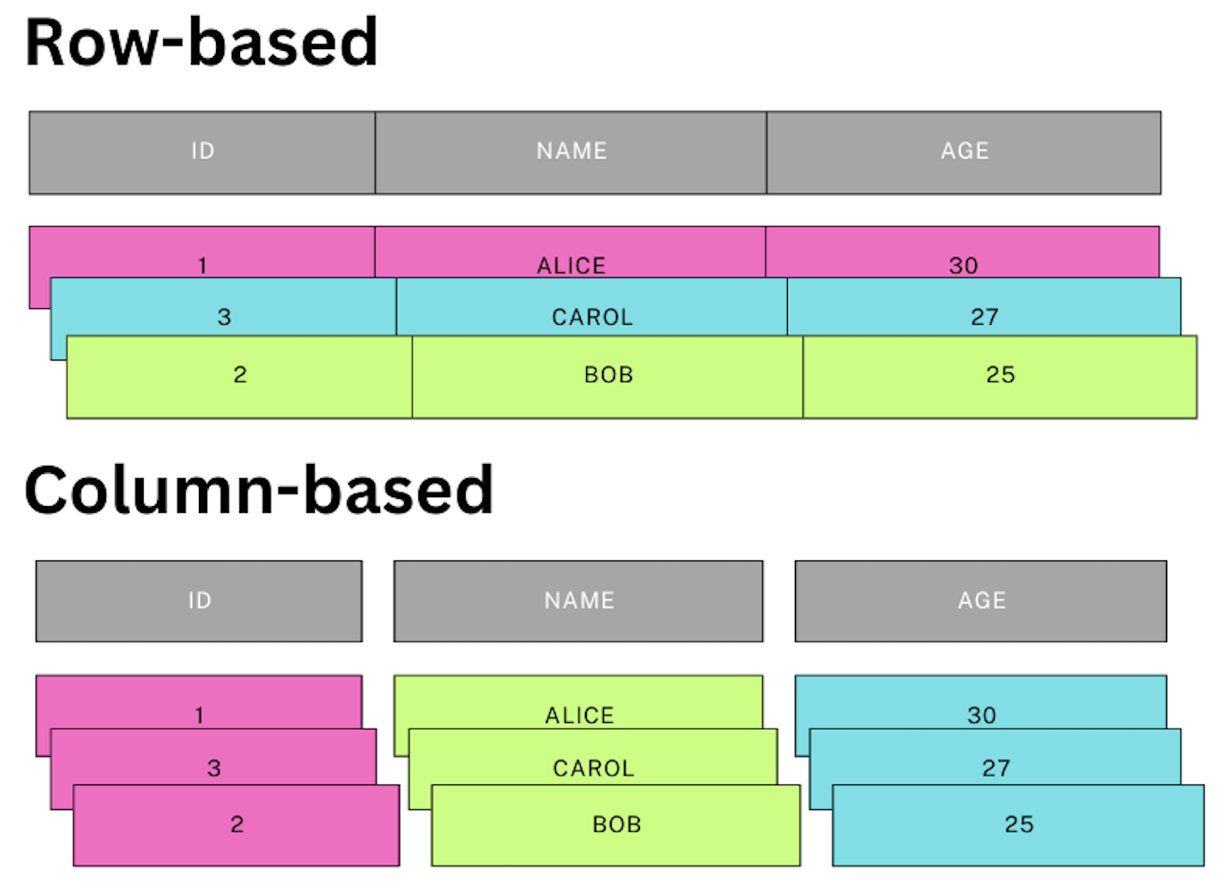
Unlike traditional row-based storage formats, where data is stored row by row, columnar storage formats store data by columns. Parquet's columnar storage layout allows for efficient data scanning and retrieval, which is particularly beneficial for analytical queries that often involve aggregating values from a specific column. This format reduces the amount of data read from disk, improving query performance and reducing I/O operations.
Understanding Columnar Storage
To illustrate the concept of columnar storage, let's consider a simple example with a dataset comprising three columns: ID, Name, and Age.
Row-Based Storage
In a row-based storage format (e.g., CSV), the data would be stored as follows:
plaintextCSV file

+----+------+-----+
| ID | Name | Age |  <- row 0 (header)
+----+------+-----+
| 1  | Alice| 30  |  <- row 1
| 2  | Bob  | 25  |  <- row 2
| 3  | Carol| 27  |  <- row 3
+----+------+-----+
In this format, each row is stored contiguously. When querying data, such as retrieving all the ages, the system has to scan through each row and extract the Age column, which can be inefficient for large datasets.
Columnar Storage
In a columnar storage format like Parquet, the same dataset is stored by columns:
plaintextID   = [1, 2, 3]
Name = [Alice, Bob, Carol]
Age  = [30, 25, 27]
In this format, each column is stored contiguously. When querying data, such as retrieving all the ages, the system can directly read the Age column, significantly reducing the amount of data read from the disk.
Suppose you come from the data engineering or analytics world. In that case, you probably have experience with queries that don’t focus on selecting one specific record from a table, but instead look for large chunks, or in some cases the entirety of the data to aggregate the values.
Advantages of Columnar Storage
There are three main advantages to using columnar storage:
- Efficient Data Retrieval: Analytical queries often need to process large volumes of data but only a subset of columns. Columnar storage allows these queries to read only the relevant columns, minimizing disk I/O and improving performance.
- Better Compression: Columns typically contain similar data types, which compress more efficiently than rows with heterogeneous data types. Parquet leverages this by applying compression techniques like run-length encoding and dictionary encoding to reduce storage space.
- Vectorized Processing: Columnar storage enables vectorized processing, where operations are applied to entire columns rather than individual rows. This approach can significantly speed up computations.
Example of Compression and Encoding
Parquet supports various compression techniques (e.g., Snappy, Gzip, LZO) and encoding schemes (e.g., RLE, dictionary encoding) to reduce storage space and enhance performance. These features help manage large datasets more effectively by minimizing disk usage and speeding up data processing.
Consider a dataset with a column Status that contains many repeated values:
plaintextStatus = [Active, Active, Active, Inactive, Inactive, Active, Active, Inactive]Using run-length encoding, Parquet would compress this column as follows:
plaintextStatus = [(Active, 3), (Inactive, 2), (Active, 2), (Inactive, 1)]This compression reduces the storage size and speeds up the processing of the Status column.
The Anatomy of a Parquet File: Structure and Optimization
Parquet by default splits data into 1GB files (this parameter is configurable), resulting in the generation of multiple .parquet files.
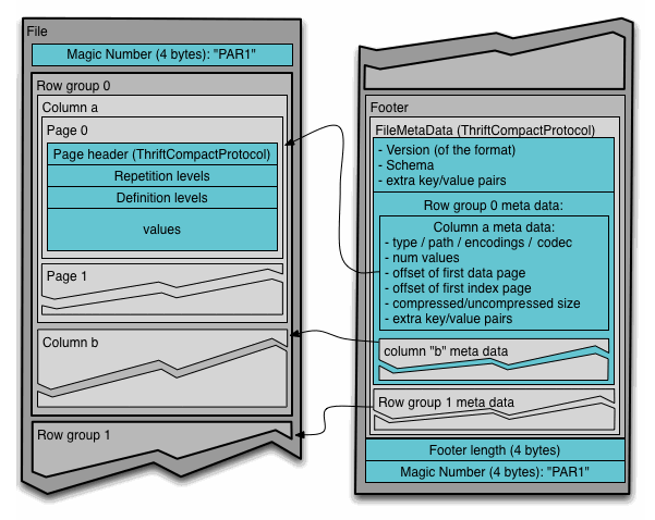
Parquet's columnar storage format is implemented through its hierarchical structure, which includes row groups, column chunks, and pages:
Row Groups
A row group is a large chunk of data that contains column data for a subset of rows. Each row group contains column chunks for each column in the dataset.
Each column in a row group has min/max statistics, allowing query engines to skip entire row groups for specific queries, resulting in significant performance gains when reading data.
Column Chunks
A column chunk stores data for a single column within a row group. Column chunks are divided into pages.
Pages
Pages are the smallest unit of data storage in Parquet. Each column chunk is divided into pages, which can be of several types:
- Data Pages: Store the actual column data.
- Dictionary Pages: Store unique values for dictionary encoding, which is a technique used to compress columns that have many repeated values.
- Index Pages: Store index information to enable faster data retrieval.
Here's a simplified representation of Parquet's structure:
plaintextParquet File

+-----------------------------+
|         Row Group 1         |
| +---------+  +---------+    |
| | Column1 |  | Column2 | ...|
| | Chunk1  |  | Chunk1  |    |
| +---------+  +---------+    |
+-----------------------------+
|         Row Group 2         |
| +---------+  +---------+    |
| | Column1 |  | Column2 | ...|
| | Chunk2  |  | Chunk2  |    |
| +---------+  +---------+    |
+-----------------------------+
Metadata
Parquet files include metadata that plays a crucial role in understanding and efficiently accessing the data they contain. This metadata is embedded within the file structure itself and typically appears in several key places:
File Header: At the beginning of a Parquet file, metadata provides essential information about the file such as its schema, compression algorithms used, and other file-level properties. This header helps software applications quickly interpret and process the file.
Row Groups: Data is organized into row groups within a Parquet file. Each row group includes its own metadata section that specifies details like the number of rows, column statistics (min/max values), and encoding used for each column. This information aids in optimizing data retrieval and query performance.
Page Metadata: Data within a row group is further divided into pages. Each data page includes metadata indicating its size, compression type, and other specifics necessary for efficient data reading and decompression.
Practical Example
Let's consider a practical example with a dataset comprising three columns: ID, Name, and Age. We'll create a Parquet file to store this data.
plaintextID  | Name  | Age
----+-------+-----
1   | Alice | 30
2   | Bob   | 25
3   | Carol | 27
4   | Dave  | 22
5   | Eve   | 29
Step-by-Step Breakdown
- Row Group Creation: Assume we decide to create one row group for this dataset.
- Column Chunks: For each column, a column chunk is created within the row group.
- Pages: Each column chunk is further divided into pages. For simplicity, let's assume each column chunk contains two pages.
Here's a simplified representation:
plaintextParquet File

+----------------------------------------------+
|                  Row Group 1                 |
| +------------+  +------------+  +------------+
| |  ID Chunk  |  | Name Chunk |  |  Age Chunk |
| | +--------+ |  | +--------+ |  | +--------+ |
| | | Page 1 | |  | | Page 1 | |  | | Page 1 | |
| | | Page 2 | |  | | Page 2 | |  | | Page 2 | |
| +------------+  +------------+  +------------+
+----------------------------------------------+
Detailed Breakdown of Pages
- ID Column Chunk:
- Page 1: Contains IDs [1, 2, 3]
- Page 2: Contains IDs [4, 5]
- Name Column Chunk:
- Page 1: Contains Names [Alice, Bob, Carol]
- Page 2: Contains Names [Dave, Eve]
- Age Column Chunk:
- Page 1: Contains Ages [30, 25, 27]
- Page 2: Contains Ages [22, 29]
Compression and Encoding
For example, if the Name column contains many repeated values, Parquet can use dictionary encoding:
- Dictionary Page: Stores unique names [Alice, Bob, Carol, Dave, Eve]
- Data Pages: Store references to the dictionary indices instead of the actual names.
Advantages of This Structure
- Efficient Data Retrieval: Analytical queries often target specific columns. For instance, if a query only needs the Age column, Parquet can read just the Age column chunks and pages, skipping ID and Name.
- Better Compression: Each column's data is typically homogeneous, allowing Parquet to use more effective compression techniques. For example, run-length encoding can compress repeated values efficiently.
- Optimized for Analytics: Parquet's columnar format is designed for read-heavy workloads typical in data analytics. It reduces the amount of data read from disk, improving query performance.
Python example
As an exercise, let’s inspect a Parquet file using Python. For this, we will use the pandas and pyarrow libraries. First, let's create a Parquet file with the example data provided, and then we'll inspect its structure.
2. Creating and Writing Data to a Parquet File
Make sure you have the necessary libraries installed. If not, you can install them using pip: pip install pandas pyarrow.
Here is a Python script to create a DataFrame with the sample data and save it as a Parquet file:
pythonimport pandas as pd

# Create a sample DataFrame
data = {
    'ID': [1, 2, 3, 4, 5],
    'Name': ['Alice', 'Bob', 'Carol', 'Dave', 'Eve'],
    'Age': [30, 25, 27, 22, 29]
}
df = pd.DataFrame(data)

# Save DataFrame to Parquet file
df.to_parquet('sample.parquet')
3. Inspecting the Parquet File
To inspect the structure of the Parquet file, including the row groups, column chunks, and pages, we can use the pyarrow library. Here’s a Python script to read and display the content and structure of the Parquet file:
pythonimport pyarrow.parquet as pq

# Read the Parquet file
parquet_file = pq.ParquetFile('sample.parquet')

# Print metadata
print("Parquet File Metadata:")
print(parquet_file.metadata)

# Print schema
print("\nParquet File Schema:")
print(parquet_file.schema)

# Inspect row groups
print("\nRow Groups:")
for i in range(parquet_file.metadata.num_row_groups):
    row_group = parquet_file.metadata.row_group(i)
    print(f"Row Group {i}:")
    print(f"  Number of rows: {row_group.num_rows}")
    for j in range(row_group.num_columns):
        column = row_group.column(j)
        print(f"  Column {j}:")
        print(f"    Name: {column.path_in_schema}")
        print(f"    Data page offset: {column.data_page_offset}")
        print(f"    Dictionary page offset: {column.dictionary_page_offset}")
        print(f"    Total compressed size: {column.total_compressed_size}")
        print(f"    Total uncompressed size: {column.total_uncompressed_size}")

# Load the DataFrame from the Parquet file to verify the content
df_loaded = pd.read_parquet('sample.parquet')
print("\nLoaded DataFrame:")
print(df_loaded)
Example Output
- Metadata and Schema: The script first prints the metadata and schema of the Parquet file, providing an overview of the file structure.
- Row Groups and Columns: It then iterates through each row group and column, displaying detailed information such as the number of rows, data page offset, dictionary page offset, and size.
- Loaded DataFrame: Finally, the script loads the data back into a DataFrame and prints it to verify the content.
Running the above script will produce an output similar to this:
pythonParquet File Metadata:
<pyarrow._parquet.FileMetaData object at 0x7f7f0c5b84f0>
  created_by: parquet-cpp-arrow version 2.0.0
  num_columns: 3
  num_rows: 5
  num_row_groups: 1
  format_version: 1.0
  serialized_size: 424

Parquet File Schema:
ID: INT64 NOT NULL
Name: BYTE_ARRAY
Age: INT64

Row Groups:
Row Group 0:
  Number of rows: 5
  Column 0:
    Name: ID
    Data page offset: 4
    Dictionary page offset: None
    Total compressed size: 63
    Total uncompressed size: 40
  Column 1:
    Name: Name
    Data page offset: 67
    Dictionary page offset: 4
    Total compressed size: 146
    Total uncompressed size: 123
  Column 2:
    Name: Age
    Data page offset: 213
    Dictionary page offset: None
    Total compressed size: 63
    Total uncompressed size: 40

Loaded DataFrame:
   ID   Name  Age
0   1  Alice   30
1   2    Bob   25
2   3  Carol   27
3   4   Dave   22
4   5    Eve   29
This structure is particularly beneficial for analytical queries and large-scale data processing, providing significant performance improvements and efficient data compression.
Data Types Supported by Apache Parquet
Parquet contains schema information in its metadata, so the query engines don’t need to infer the schema or the user doesn’t need to specify it when reading the data manually.
Parquet supports a wide range of data types, including primitive types (e.g., INT32, FLOAT) and complex types (e.g., structs, arrays). This versatility makes it suitable for diverse data structures encountered in modern applications.
The supported primitive data types are:
BOOLEAN: 1-bit Boolean.INT32: 32-bit signed integer.INT64: 64-bit signed integer.INT96: 96-bit signed integer.FLOAT: IEEE 32-bit floating point.DOUBLE: IEEE 64-bit floating point.BYTE_ARRAY: Array of bytes of arbitrary length.FIXED_LEN_BYTE_ARRAY: Fixed-length byte array.
The Parquet approach involves using the minimum number of primitive data types. It utilizes logical types to expand on these primitive types, specifying how they should be interpreted through annotations. For instance, a string is depicted as a byte_array with the UTF8 annotation.
Here's a realistic example to illustrate the supported data types:
pythonmessage User {
  required int32 UserId;
  required binary Name (UTF8);
  optional binary Email (UTF8);
  optional int32 Age;
  optional group Address {
    required binary Street (UTF8);
    required binary City (UTF8);
    required int32 ZipCode;
  }
  repeated binary PhoneNumbers (UTF8);
}
And a sample of the dataset, which demonstrates how Parquet can store repeated, optional values too.
pythonUserId  Name   Email              Age  Address                     PhoneNumbers
1       Alice  alice@e.com  30   1 M St, Anytown, 12345      [123-456-7890,555-123-4567]
2       Bob    bob@e.com    25   2 M Ave, Othertown, 67890   [987-654-3210]
3       Carol  carol@e.com  27   3 O Dr, Thistown, 11223
Example of Nested Data Structure:
pythonAddress Group:

+------------------------+
|       Address          |
| +--------+  +-------+  |
| | Street |  | City  |  |
| +--------+  +-------+  |
| | Main   |  | Any   |  |
| | Maple  |  | Other |  |
| | Oak    |  | This  |  |
| +--------+  +-------+  |
| +----------+           |
| | ZipCode  |           |
| +----------+           |
| | 12345    |           |
| | 67890    |           |
| | 11223    |           |
| +----------+           |
+------------------------+
Example of Repeated Field (PhoneNumbers):
pythonPhoneNumbers:

+---------------------+
| PhoneNumber         |
+---------------------+
| 123-456-7890        |
| 555-123-4567        |
| 987-654-3210        |
| (empty for Carol)   |
+---------------------+
By supporting complex types like structs and arrays, Parquet can efficiently store and query nested and repeated data structures, making it suitable for a wide range of applications, from simple tabular data to complex hierarchical data models.
Writing Data to Parquet: A Step-by-Step Guide (with Python Example)
Let’s take a deeper look at what it takes to write data into a Parquet file. These steps include preparing the schema, organizing the data into row groups and column chunks, compressing and encoding the data, and writing the metadata and data to the file. Keep in mind that Parquet files are immutable.
We’re going to use pyarrow in the examples due to its popularity and comprehensive support for working with Parquet files in Python. It is a robust library maintained by the Apache Arrow project, designed for high-performance in-memory data processing, and provides seamless interoperability between different data processing frameworks.
However, if you prefer a different library or want to demonstrate the functionality with another tool take a look at fastparquet.
1. Defining the Schema
The first step is to define the schema of the data to be written. This schema includes information about the column names, data types, and any nested structures.
pythonSchema Definition

+-----------------------------+
| Column Name | Data Type     |
|-------------|---------------|
| UserId      | INT64         |
| Name        | STRING        |
| Age         | INT32         |
|-----------------------------+
Example in Python:
pythonimport pyarrow as pa

# Define the schema
schema = pa.schema([
    ('UserId', pa.int64()),
    ('Name', pa.string()),
    ('Age', pa.int32())
])
2. Organizing Data into Row Groups
Data is organized into row groups, with each row group containing data for a subset of rows. This step includes partitioning the data into manageable chunks.t
pythonRow Groups
+-----------------------------+
|         Row Group 1         |
| +---------+  +---------+    |
| | UserId  |  | Name    |    |
| | 1       |  | Alice   |    |
| | 2       |  | Bob     |    |
| +---------+  +---------+    |
| Age: 30, 25                 |
+-----------------------------+
|         Row Group 2         |
| +---------+  +---------+    |
| | UserId  |  | Name    |    |
| | 3       |  | Carol   |    |
| | 4       |  | Dave    |    |
| +---------+  +---------+    |
| Age: 27, 22                 |
+-----------------------------+
Python example with pyarrow:
python# Create data for the table
data = [
    pa.array([1, 2, 3, 4], type=pa.int64()),
    pa.array(['Alice', 'Bob', 'Carol', 'Dave'], type=pa.string()),
    pa.array([30, 25, 27, 22], type=pa.int32())
]

# Create a table with the schema
table = pa.Table.from_arrays(data, schema=schema)
3. Compressing and Encoding Data
Each column chunk within the row groups is compressed and encoded to optimize storage and retrieval.
pythonColumn Chunks
+-----------------------------+
|         Column1 (UserId)    |
| +---------+  +---------+    |
| | Value 1 |  | Value 2 |    |
| +---------+  +---------+    |
| Compression: SNAPPY         |
| Encoding: PLAIN             |
+-----------------------------+
|         Column2 (Name)      |
| +---------+  +---------+    |
| | Value 1 |  | Value 2 |    |
| +---------+  +---------+    |
| Compression: SNAPPY         |
| Encoding: PLAIN             |
+-----------------------------+
Python example:
pythonimport pyarrow.parquet as pq

# Define the compression and encoding options
compression = 'SNAPPY'

# Write the table to a Parquet file with the specified compression
pq.write_table(table, 'data.parquet', compression=compression)
4. Writing Metadata and Data
The final step involves writing the metadata and the compressed, encoded data to the Parquet file. This includes writing the schema, row group information, column chunk details, and the actual data pages.
pythonParquet File

+-----------------------------+
|         File Header         |
| +-------------------------+ |
| |       Magic Number      | |
| +-------------------------+ |
|         Row Group 1         |
| +---------+  +---------+    |
| | Column1 |  | Column2 |    |
| | Chunk1  |  | Chunk1  |    |
| +---------+  +---------+    |
+-----------------------------+
|         Row Group 2         |
| +---------+  +---------+    |
| | Column1 |  | Column2 |    |
| | Chunk2  |  | Chunk2  |    |
| +---------+  +---------+    |
+-----------------------------+
|         File Footer         |
| +-------------------------+ |
| |       Metadata          | |
| +-------------------------+ |
+-----------------------------+
The previous pq.write_table call already handles writing metadata and data to the file.
Full Python Example
Here’s a complete Python example demonstrating the steps to write data to a Parquet file using the pyarrow library:
pythonimport pyarrow as pa
import pyarrow.parquet as pq

# Step 1: Define the schema
schema = pa.schema([
    ('UserId', pa.int64()),
    ('Name', pa.string()),
    ('Age', pa.int32())
])

# Step 2: Create data for the table
data = [
    pa.array([1, 2, 3, 4], type=pa.int64()),
    pa.array(['Alice', 'Bob', 'Carol', 'Dave'], type=pa.string()),
    pa.array([30, 25, 27, 22], type=pa.int32())
]

# Create a table with the schema
table = pa.Table.from_arrays(data, schema=schema)

# Step 3: Define the compression and encoding options
compression = 'SNAPPY'

# Step 4: Write the table to a Parquet file with the specified compression
pq.write_table(table, 'data.parquet', compression=compression)
Not that complicated, right? Let’s take a look at the flipside – how do we read from a Parquet file?
Reading Parquet Files: A Comprehensive Tutorial (with Python Example)
Reading data from a Parquet file also involves several steps, each designed to optimize data retrieval and minimize I/O operations.
Let’s break them down.
1. Opening the Parquet File
The process begins with opening the Parquet file. This is akin to accessing any file stored on a local disk, a distributed file system (like HDFS), or cloud storage.
2. Reading Parquet File Metadata
The next step is to read the metadata located in the file footer, which includes schema information, row group details, and column metadata.
pythonParquet File

+-----------------------------+
|         File Footer         |
| +-------------------------+ |
| |       Metadata          | |
| | +---------------------+ | |
| | | Schema Information  | | |
| | | Row Groups Info     | | |
| | | Column Metadata     | | |
| | +---------------------+ | |
| +-------------------------+ |
+-----------------------------+
Example in Python:
pythonimport pyarrow.parquet as pq

# Open the Parquet file
parquet_file = pq.ParquetFile('data.parquet')

# Read the file metadata
metadata = parquet_file.metadata
print("Schema:")
print(metadata.schema)
3. Selecting Row Groups
Based on the metadata, row groups are selected. Predicate pushdown can be used to filter out unnecessary row groups.
pythonParquet File

+-----------------------------+
|         Row Groups          |
| +---------+  +-----------+  |
| |RowGroup1|  | RowGroup2 |  |
| +---------+  +-----------+  |
|  (Apply filters to select   |
|    relevant row groups)     |
+-----------------------------+
4. Reading Column Chunks
Within each selected row group, column chunks are identified and read. Only the required columns are accessed.
pythonSelected Row Group

+-----------------------------+
|         Row Group 1         |
| +---------+  +---------+    |
| | Column1 |  | Column2 |    |
| | Chunk1  |  | Chunk1  |    |
| +---------+  +---------+    |
|   (Read only the required   |
|    columns for the query)   |
+-----------------------------+
Python example:
python# Select the columns to read
columns_to_read = ['UserId', 'Name', 'Age']

# Read the data into a table
table = parquet_file.read(columns=columns_to_read)
5. Decompressing and Decoding Pages
Each column chunk consists of pages, which are decompressed and decoded as needed.
pythonColumn Chunk (Column1)
+-----------------------------+
|         Pages               |
| +---------+  +---------+    |
| | Page1   |  | Page2   |    |
| +---------+  +---------+    |
| (Decompress and decode      |
|   pages as needed)          |
+-----------------------------+
6. Materializing Rows
Finally, the decompressed and decoded data is materialized into rows as required by the query.
python+-----------------------------+
|       Materialized Rows     |
| +-------+  +-------+ +------+
| | UserId|  | Name  |  Age   |
| | 1     |  | Alice |   30   |
| | 2     |  | Bob   |   25   |
| | 3     |  | Carol |   27   |
| +-------+  +-------+ +------+
+-----------------------------+
Python example:
pythonimport pandas as pd

# Convert the table to a pandas DataFrame for easy manipulation
df = table.to_pandas()

# Display the DataFrame
print(df)
Full Python Example
Here’s how all these steps come together in a full Python example using the pyarrow library:
pythonimport pyarrow.parquet as pq
import pandas as pd

# Step 1: Open the Parquet file
parquet_file = pq.ParquetFile('data.parquet')

# Step 2: Read the file metadata
metadata = parquet_file.metadata
print("Schema:")
print(metadata.schema)

# Step 3: Select the columns to read
columns_to_read = ['UserId', 'Name', 'Age']

# Step 4: Read the data into a table (automatically selects and reads row groups and column chunks)
table = parquet_file.read(columns=columns_to_read)

# Step 5: (Handled internally) Decompress and decode pages

# Step 6: Materialize rows by converting the table to a pandas DataFrame
df = table.to_pandas()

# Display the DataFrame
print(df)
This process highlights how Parquet's structure and metadata enable efficient data reading, tailored to the specific needs of each query.
Apache Parquet: Advantages and Limitations
To recap, let’s take a look at the pros and cons of Parquet.
Pros
- Efficient data compression and encoding reduce storage requirements.
- Columnar format enhances performance for analytical queries.
- Schema evolution support allows flexibility in data modeling.
- Widely supported across various data processing tools and frameworks.
Cons
- Initial setup and integration can be complex for beginners.
- Not ideal for small, transactional datasets due to the overhead of managing row groups and pages.
- Writing data into Parquet might be slower slower than other storage formats.
- Parquet is a binary format, which makes it not human-readable.
Conclusion
Apache Parquet has become a critical component in the data storage and analytics industry. Its efficient columnar storage format, compression features, and ability to support schema evolution make it a valuable tool for handling large amounts of data.
As the demand for data processing continues to increase, Parquet's role in facilitating high-performance, cost-effective analytics is expected to grow. By harnessing its strengths, organizations can significantly improve their data processing workflows and extract deeper insights from their data.

About the author
Dani is a data professional with a rich background in data engineering and real-time data platforms. At Estuary, Daniel focuses on promoting cutting-edge streaming solutions, helping to bridge the gap between technical innovation and developer adoption. With deep expertise in cloud-native and streaming technologies, Dani has successfully supported startups and enterprises in building robust data solutions.

